Analysis of mutational signatures with musicatk in the R console

Introduction

A variety of exogenous exposures or endogenous biological processes can contribute to the overall mutational load observed in human tumors. Many different mutational patterns, or “mutational signatures”, have been identified across different tumor types. These signatures can provide a record of environmental exposure and can give clues about the etiology of carcinogenesis. The Mutational Signature Comprehensive Analysis Toolkit (musicatk) contains a complete end-to-end workflow for characterization of mutational signatures in a cohort of samples. musicatk has utilities for extracting variants from a variety of file formats, multiple methods for discovery of novel signatures or prediction of pre-existing signatures, and many types of downstream visualizations for exploratory analysis. This package has the ability to parse and combine multiple motif classes in the mutational signature discovery or prediction processes. Mutation motifs include single base substitutions (SBS), double base substitutions (DBS), insertions (INS) and deletions (DEL). The package can be loaded using the library command:

library(musicatk)

Importing mutational data

In order to discover or predict mutational signatures, we must first set up our musica object by 1) extracting variants from files or objects such as VCFs and MAFs, 2) selecting the appropriate reference genome 3) creating a musica object, 4) adding sample-level annotations, and 5) building a count tables for our variants of interest. Alternatively, a musica object can be created directly from a count table.

Import variants from files

Variants can be extracted from various formats using the following functions:

The extract_variants_from_vcf_file() function will extract variants from a VCF file. The file will be imported using the readVcf function from the VariantAnnotation package and then the variant information will be extracted from this object.
The extract_variants_from_vcf() function extracts variants from a CollapsedVCF or ExpandedVCF object from the VariantAnnotation package.
The extract_variants_from_maf_file() function will extract variants from a file in Mutation Annotation Format (MAF) used by TCGA.
The extract_variants_from_maf() function will extract variants from a MAF object created by the maftools package.
The extract_variants_from_matrix() function will get the information from a matrix or data.frame like object that has columns for the chromosome, start position, end position, reference allele, mutation allele, and sample name.
The extract_variants() function will extract variants from a list of objects. These objects can be any combination of VCF files, VariantAnnotation objects, MAF files, MAF objects, and data.frame objects.

Below are some examples of extracting variants from MAF and VCF files:

# Extract variants from a MAF File
lusc_maf <- system.file("extdata", "public_TCGA.LUSC.maf", package = "musicatk")
lusc.variants <- extract_variants_from_maf_file(maf_file = lusc_maf)

# Extract variants from an individual VCF file
luad_vcf <- system.file("extdata", "public_LUAD_TCGA-97-7938.vcf",
  package = "musicatk"
)
luad.variants <- extract_variants_from_vcf_file(vcf_file = luad_vcf)

# Extract variants from multiple files and/or objects
melanoma_vcfs <- list.files(system.file("extdata", package = "musicatk"),
  pattern = glob2rx("*SKCM*vcf"), full.names = TRUE
)
variants <- extract_variants(c(lusc_maf, luad_vcf, melanoma_vcfs))

Import TCGA datasets

For this tutorial, we will analyze mutational data from lung and skin tumors from TCGA. This data will be retrieved using the the GDCquery function from TCGAbiolinks package.

library(TCGAbiolinks)
tcga_datasets <- c("TCGA-LUAD", "TCGA-LUSC", "TCGA-SKCM")
types <- gsub("TCGA-", "", tcga_datasets)

variants <- NULL
annot <- NULL
for (i in seq_along(tcga_datasets)) {
  # Download variants
  query <- GDCquery(
    project = tcga_datasets[i],
    data.category = "Simple Nucleotide Variation",
    data.type = "Masked Somatic Mutation",
    workflow.type = "Aliquot Ensemble Somatic Variant Merging and Masking",
    experimental.strategy = "WXS",
    data.format = "maf"
  )
  GDCdownload(query)
  data <- GDCprepare(query)

  # Extract from maf
  temp <- extract_variants_from_matrix(data)
  variants <- rbind(variants, temp)
  annot <- rbind(annot, cbind(
    rep(types[i], length(unique(temp$sample))),
    unique(as.character(temp$sample))
  ))
}
colnames(annot) <- c("Tumor_Type", "ID")
rownames(annot) <- annot[, "ID"]

Note that with previous versions of the GDC database, you may need to set worflow.type to another string such as workflow.type = MuTect2 Variant Aggregation and Masking.

Creating a musica object

A genome build must first be selected before a musica object can be created for mutational signature analysis. musicatk uses BSgenome objects to access genome sequence information that flanks each mutation which is used bases for generating mutation count tables. BSgenome objects store full genome sequences for different organisms. A full list of supported organisms can be obtained by running available.genomes() after loading the BSgenome library. Custom genomes can be forged as well (see BSgenome documentation). musicatk provides a utility function called select_genome() to allow users to quickly select human genome build versions “hg19” and “hg38” or mouse genome builds “mm9” and “mm10”. The reference sequences for these genomes are in UCSC format (e.g. chr1).

g <- select_genome("hg38")

The last preprocessing step is to create an object with the variants and the genome using the create_musica_from_variants function. This function will perform checks to ensure that the chromosome names and reference alleles in the input variant object match those in supplied BSgenome object. These checks can be turned off by setting check_ref_chromosomes = FALSE and check_ref_bases = FALSE, respectively. This function also looks for adjacent single base substitutions (SBSs) and will convert them to double base substitutions (DBSs). To disable this automatic conversion, set convert_dbs = FALSE.

musica <- create_musica_from_variants(x = variants, genome = g)

## Checking that chromosomes in the 'variant' object match chromosomes in the 'genome' object.

## Checking that the reference bases in the 'variant' object match the reference bases in the 'genome' object.

## Standardizing INS/DEL style

## Removing 22 compound insertions

## Removing 167 compound deletions

## Converting 44 insertions

## Converting 246 deletions

## Converting adjacent SBS into DBS

## 15176 SBS converted to DBS

Importing sample annotations

Sample-level annotations, such as tumor type, treatment, or outcome can be used in downstream analyses. Sample annotations that are stored in a vector or data.frame can be directly added to the musica object using the samp_annot function:

id <- as.character(sample_names(musica))
samp_annot(musica, "Tumor_Type") <- annot[id, "Tumor_Type"]

Note: Be sure that the annotation vector or data.frame being supplied is in the same order as the samples in the musica object. The sample_names function can be used to get the order of the samples in the musica object. Note that the annotations can also be added later on.

Creating mutation count tables

Create standard tables

Motifs are the building blocks of mutational signatures. Motifs themselves are a mutation combined with other genomic information. For instance, SBS96 motifs are constructed from an SBS mutation and one upstream and one downstream base sandwiched together. We build tables by counting these motifs for each sample.

build_standard_table(musica, g = g, table_name = "SBS96")

## Building count table from SBS with SBS96 schema

Here is a list of mutation tables that can be created by setting the table_name parameter in the build_standard_table function:

SBS96 - Motifs are the six possible single base pair mutation types times the four possibilities each for upstream and downstream context bases (464 = 96 motifs)
SBS192_Trans - Motifs are an extension of SBS96 multiplied by the transcriptional strand (translated/untranslated), can be specified with "Transcript_Strand".
SBS192_Rep - Motifs are an extension of SBS96 multiplied by the replication strand (leading/lagging), can be specified with "Replication_Strand".
DBS - Motifs are the 78 possible double-base-pair substitutions
INDEL - Motifs are 83 categories intended to capture different categories of indels based on base-pair change, repeats, or microhomology, insertion or deletion, and length.

Combine tables

Different count tables can be combined into one using the combine_count_tables function. For example, the SBS96 and the DBS tables could be combined and mutational signature discovery could be performed across both mutations modalities. Tables with information about the same types of variants (e.g. two related SBS tables) should generally not be combined and used together.

# Build Double Base Substitution table
build_standard_table(musica, g = g, table_name = "DBS78")

## Building count table from DBS with DBS78 schema

# Combine with SBS table
combine_count_tables(musica, to_comb = c("SBS96", "DBS78"), name = "SBS_DBS",
                     description =
                       "An example combined table, combining SBS96 and DBS")

# View all tables
names(tables(musica))

## [1] "SBS96"   "DBS78"   "SBS_DBS"

Creating a musica object directly from a count table

If a count table is already available, a musica object can be created directly without need for a variant file and building tables.

luad_count_table_path <- system.file("extdata", "luad_tcga_count_table.csv",
  package = "musicatk"
)
luad_count_table <- as.matrix(read.csv(luad_count_table_path))

musica_from_counts <- create_musica_from_counts(luad_count_table, "SBS96")

Filtering samples

Samples with low numbers of mutations should usually be excluded from discover and prediction procedures. The subset_musica_by_counts function can be used to exclude samples with low numbers of mutations in a particular table:

musica_filter <- subset_musica_by_counts(musica, table_name = "SBS96",
                                         num_counts = 10)

The subset_musica_by_annotation function can also be used to subset the musica object to samples that match a particular annotation. For example, if we only wanted to analyze lung cancer, we could filter to samples that have “LUAD” or “LUSC”:

musica_luad <- subset_musica_by_annotation(musica, annot_col = "Tumor_Type",
                                           annot_names = c("LUAD", "LUSC"))

Discovery of signatures and exposures

Mutational signature discovery is the process of deconvoluting a matrix containing the count of each mutation type in each sample into two matrices: 1) a Signature matrix containing the probability of each mutation motif in signature and 2) an Exposure matrix containing the estimated counts of each signature in each sample. Discovery and prediction results are saved in the result_list slot of a musica object. The discover_signatures function can be used to identify signatures in a dataset de novo.

Determining an appropriate k value

The k value is the number of signatures that are predicted from a discovery method. To help determine an appropriate k value, the compare_k_vals function can be used to compare to the stability and error associated with various k values. Generally, 100 replicates is suggested, as well as a larger span of k values to test. Here, fewer k values and replicates are used for simplicity.

k_comparison <- compare_k_vals(musica, "SBS96",
  reps = 100, min_k = 2, max_k = 6,
  algorithm = "lda"
)

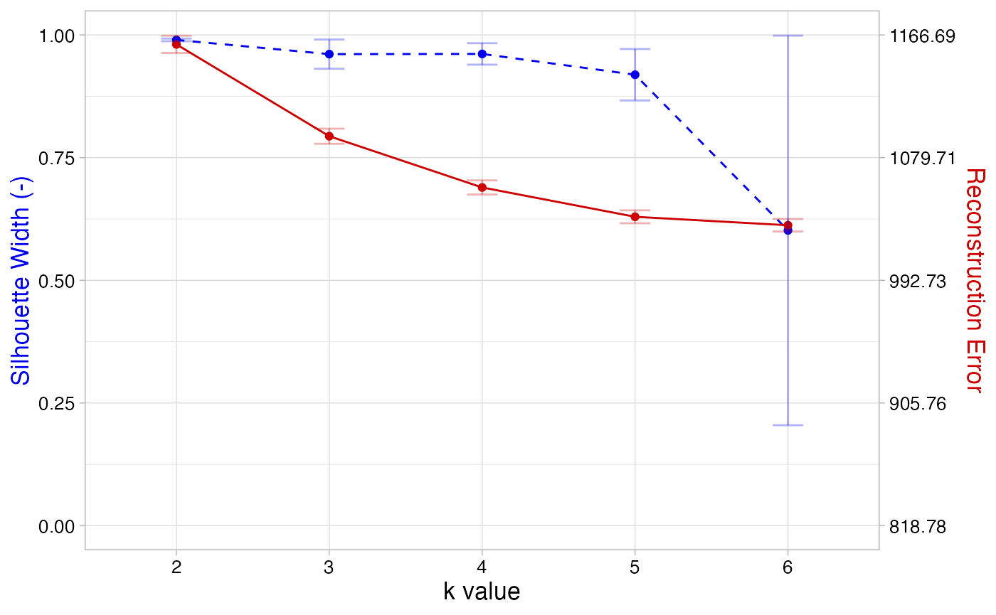
From the resulting plot, we see that k = 4 yields a relatively high silhouette width and a relatively low reconstruction error. The error bars for both metrics are also quite narrow for k = 4. Therefore four signatures should be selected, so we will set k equal to 4 in the discover_signatures function:

discover_signatures(musica_filter,
  modality = "SBS96", num_signatures = 4,
  algorithm = "lda", model_id = "ex_result"
)

Supported signature discovery algorithms include:

Non-negative matrix factorization (nmf)
Latent Dirichlet Allocation (lda)

Both have built-in seed capabilities for reproducible results, nstarts for multiple independent chains from which the best final result will be chosen. NMF also allows for parallel processing via par_cores. To get the signatures or exposures from the result object, the following functions can be used:

# Extract the exposure matrix
expos <- exposures(musica_filter, "result", "SBS96", "ex_result")
expos[1:3, 1:3]

##            TCGA-99-8033-01A-11D-2238-08 TCGA-99-8032-01A-11D-2238-08
## Signature1                    106.52551                    285.88771
## Signature2                     44.75862                     53.23718
## Signature3                      7.65405                     10.74107
##            TCGA-99-8028-01A-11D-2238-08
## Signature1                  370.2086953
## Signature2                   21.8723410
## Signature3                    0.8796583

# Extract the signature matrix
sigs <- signatures(musica_filter, "result", "SBS96", "ex_result")
sigs[1:3, 1:3]

##         Signature1  Signature2   Signature3
## C>A_ACA 0.03277323 0.004306005 5.521593e-04
## C>A_ACC 0.02966502 0.005984863 3.379481e-04
## C>A_ACG 0.02146643 0.002121666 1.519013e-05

Visualization of results

Plot signatures

The plot_signatures function can be used to display barplots that show the probability of each mutation type in each signature:

plot_signatures(musica_filter, "ex_result")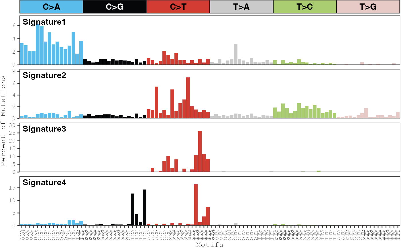

By default, the scales on the y-axis are forced to be the same across all signatures. This behavior can be turned off by setting same_scale = FALSE:

plot_signatures(musica_filter, "ex_result", same_scale = FALSE)

Comparing to external signatures

A common analysis is to compare the signatures estimated in a dataset to those generated in other datasets or to those in the COSMIC database. We have a set of functions that can be used to easily perform pairwise correlations between signatures. The compare_results functions compares the signatures between two models in the same or different musica objects. The compare_cosmic_v2 will correlate the signatures between a model and the SBS signatures in COSMIC V2. For example:

compare_cosmic_v2(musica_filter, "ex_result", threshold = 0.8)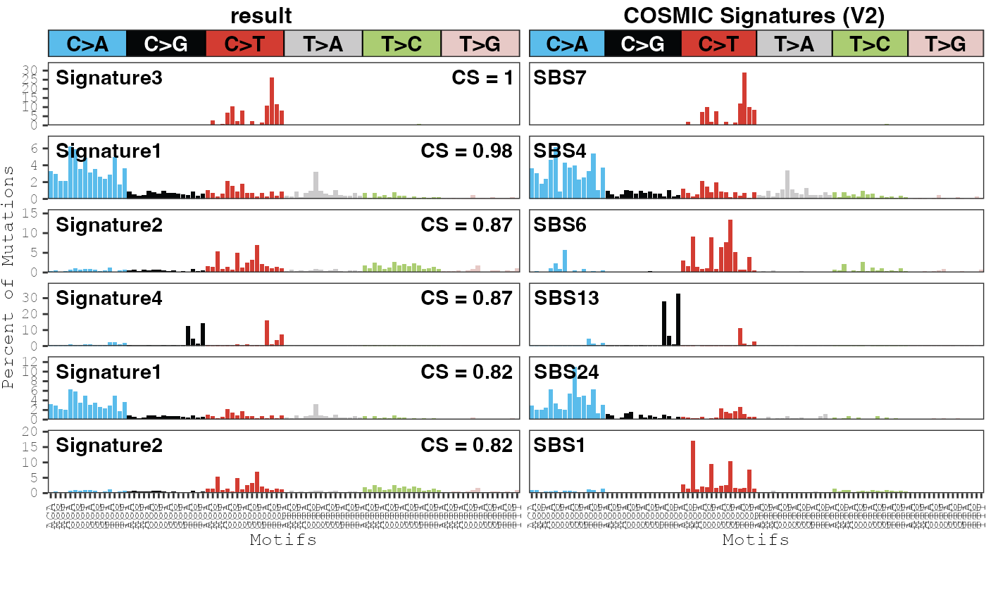

##      cosine x_sig_index y_sig_index x_sig_name y_sig_name
## 5 0.9964997           3           7 Signature3       SBS7
## 1 0.9753047           1           4 Signature1       SBS4
## 4 0.8698311           2           6 Signature2       SBS6
## 6 0.8679439           4          13 Signature4      SBS13
## 2 0.8207367           1          24 Signature1      SBS24
## 3 0.8165057           2           1 Signature2       SBS1

In this example, our Signatures 1 and 3 were most highly correlated to COSMIC Signature 4 and 7, respectively, so this may indicate that samples in our dataset were exposed to UV radiation or cigarette smoke. Only pairs of signatures who have a correlation above the threshold parameter will be returned. If no pairs of signatures are found, then you may want to consider lowering the threshold. Signatures can also be correlated to those in the COSMIC V3 database using the compare_cosmic_v3 function.

Based on the COSMIC comparison results and our prior knowledge, these signatures can be re-named and the new name can displayed in the plots:

name_signatures(musica_filter, "ex_result",
                c("SBS4 - Smoking", "SBS15 - MMR", "SBS7 - UV",
                  "SBS2/13 - APOBEC"))
plot_signatures(musica_filter, "ex_result")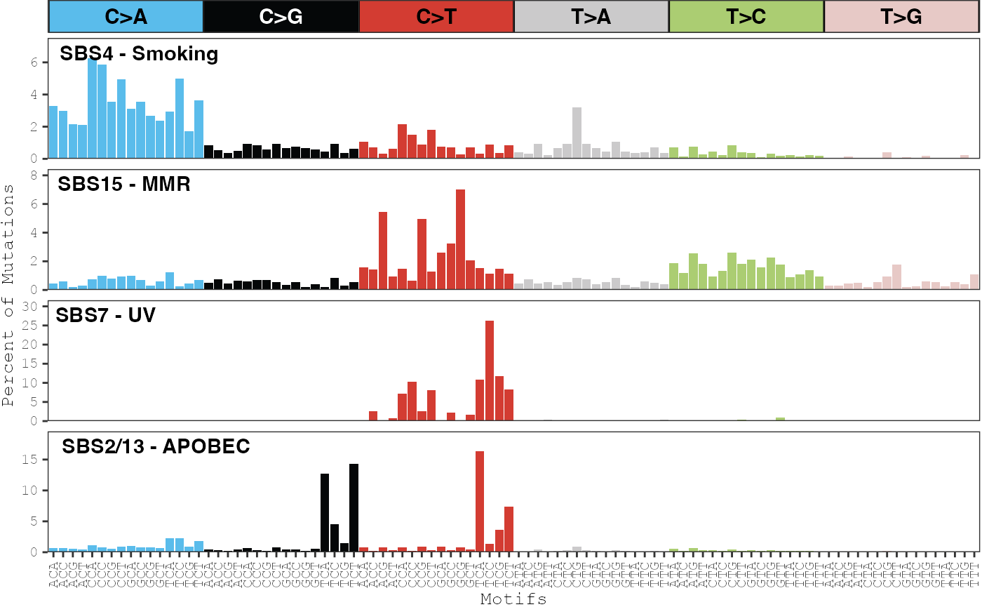

Plot exposures

Barplots showing the exposures in each sample can be plotted with the plot_exposures function:

plot_exposures(musica_filter, "ex_result", plot_type = "bar")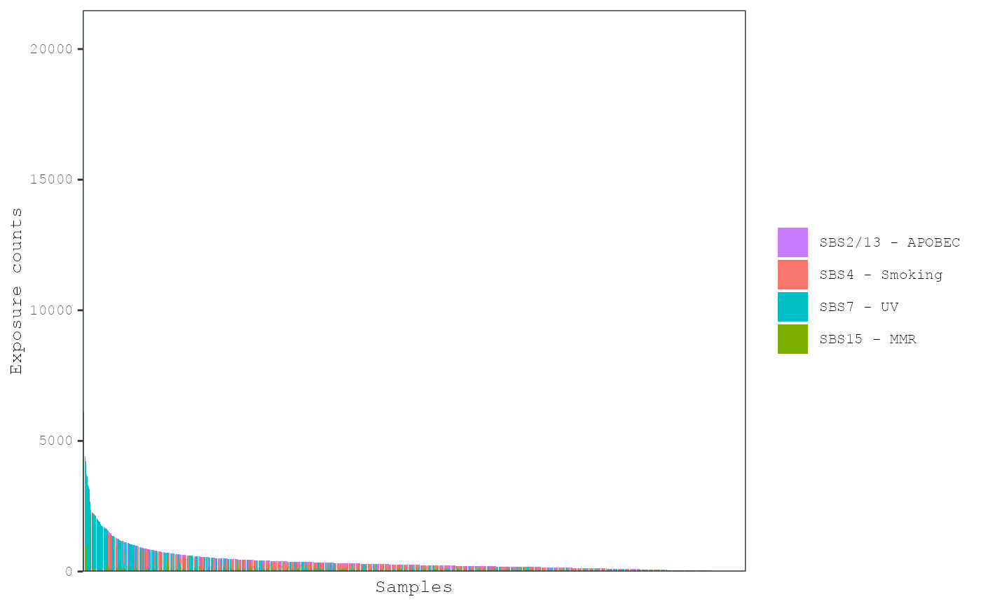

By default, samples are ordered from those with the highest number of mutations on the left to those with the lowest on the right. Sometimes, too many samples are present and the bars are too small to clearly examine the patterns of exposures. The num_samples parameter can be used to display the top samples with the highest number of mutations on the left:

plot_exposures(musica_filter, "ex_result", plot_type = "bar", num_samples = 50)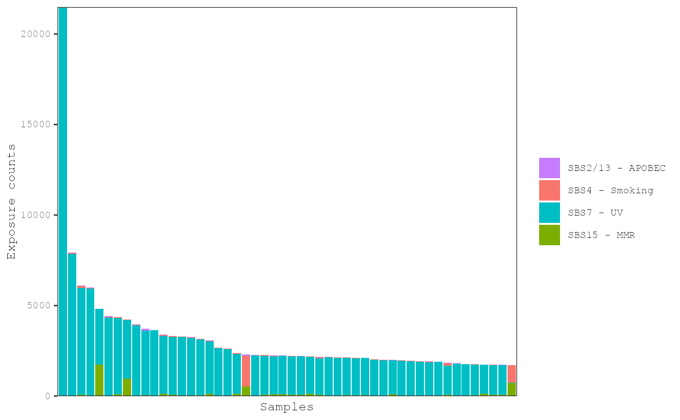

Samples can be ordered by the level of individual exposures. The can be used in combination with the num_samples parameter to examine the mutational patterns in the samples with the highest levels of a particular exposure. For example, samples can be ordered by the number of estimated mutations from the MMR signature:

plot_exposures(musica_filter, "ex_result", plot_type = "bar", num_samples = 50,
               sort_samples = "SBS15 - MMR")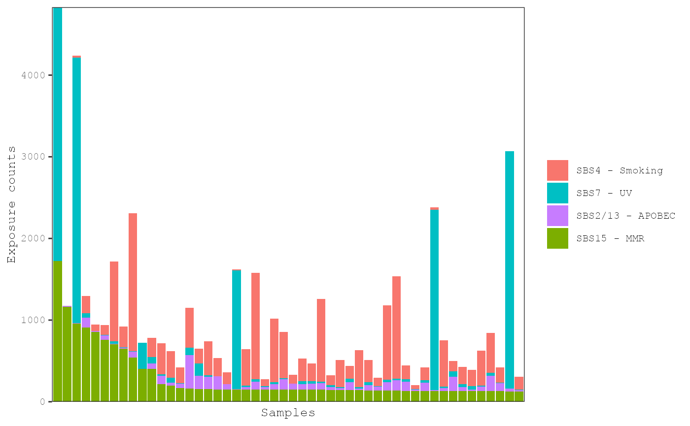

The proportion of each exposure in each tumor can be shown by setting proportional = TRUE:

plot_exposures(musica_filter, "ex_result", plot_type = "bar", num_samples = 50,
               proportional = TRUE)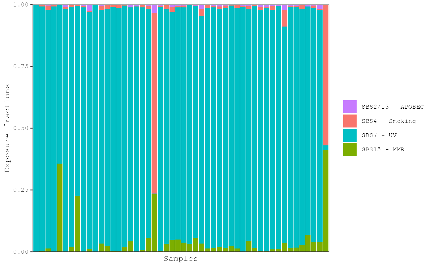

The plot_exposures function can group exposures by either a sample annotation or by a signature by setting the group_by parameter. To group by an annotation, the groupBy parameter must be set to "annotation" and the name of the annotation must be supplied via the annotation parameter. For example, the exposures from the previous result can be grouped by the Tumor_Type annotation:

plot_exposures(musica_filter, "ex_result", plot_type = "bar",
               group_by = "annotation", annotation = "Tumor_Type")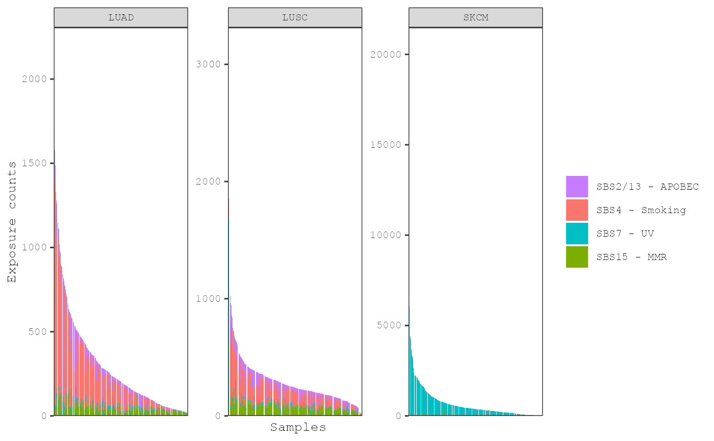

In this plot, it is clear that the smoking signature is more active in the lung cancers while the UV signature is more active in the skin cancers. The distribution of exposures with respect to annotation can be viewed using boxplots by setting plot_type = "box" and group_by = "annotation":

plot_exposures(musica_filter, "ex_result", plot_type = "box",
               group_by = "annotation", annotation = "Tumor_Type")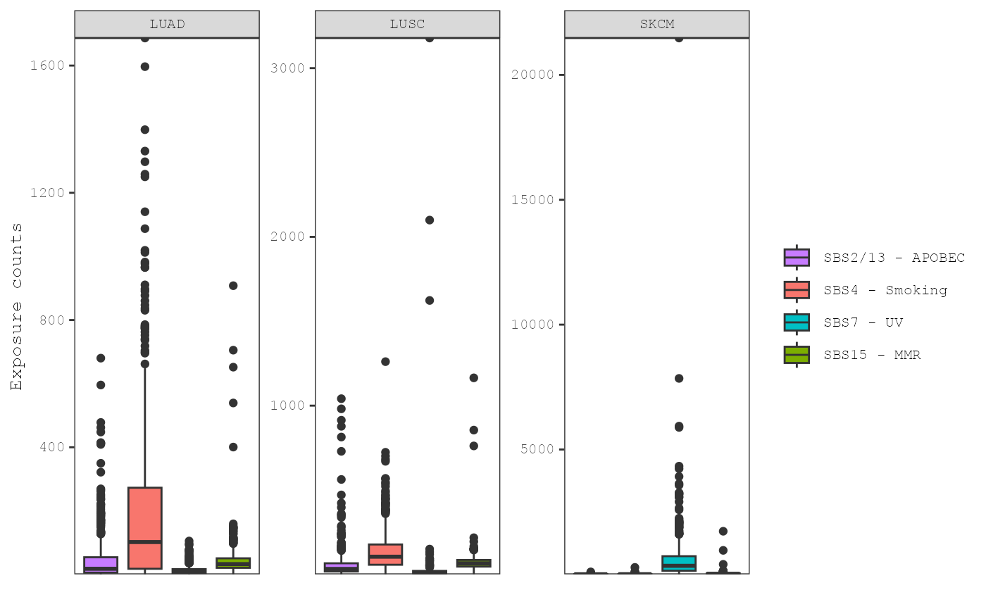

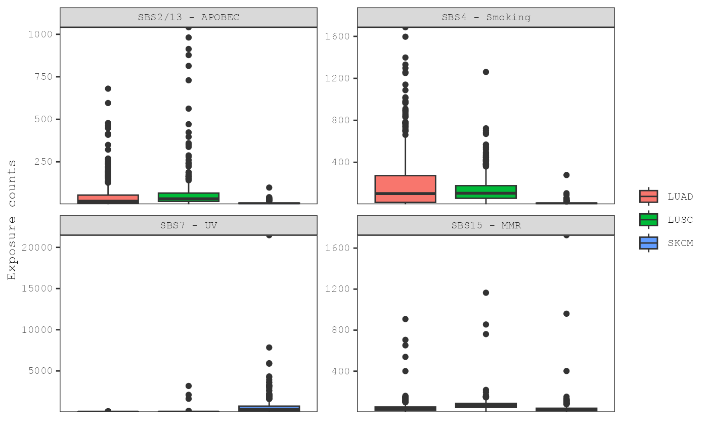
Note that boxplots can be converted to violin plots by setting plot_type = "violin". To compare the exposures levels across groups of samples within a signature, we can set group_by = "signature" and color_by = "annotation":

plot_exposures(musica_filter, "ex_result",
  plot_type = "box", group_by = "signature",
  color_by = "annotation", annotation = "Tumor_Type"
)

To verify that the deconvolution algorithm produced good signatures, one strategy is to examine the patterns of mutations in individual samples with a high predicted percentage of a particular signature. If the shape of the counts match the patterns of the signature, then this is a good indicator that the deconvolution algorithm worked well. Counts for individual samples can be plotted with the plot_sample_counts function. For example, we can plot the sample with the highest proportion of the APOBEC signature:

# Normalize exposures
expos.prop <- prop.table(expos, margin = 2)

# Plot counts for the sample with the higest level of exposures for sigs #2
# and #4
ix <- c(which.max(expos.prop[2, ]), which.max(expos.prop[4, ]))
plot_sample_counts(musica_filter, sample_names = colnames(expos.prop)[ix],
                   modality = "SBS96")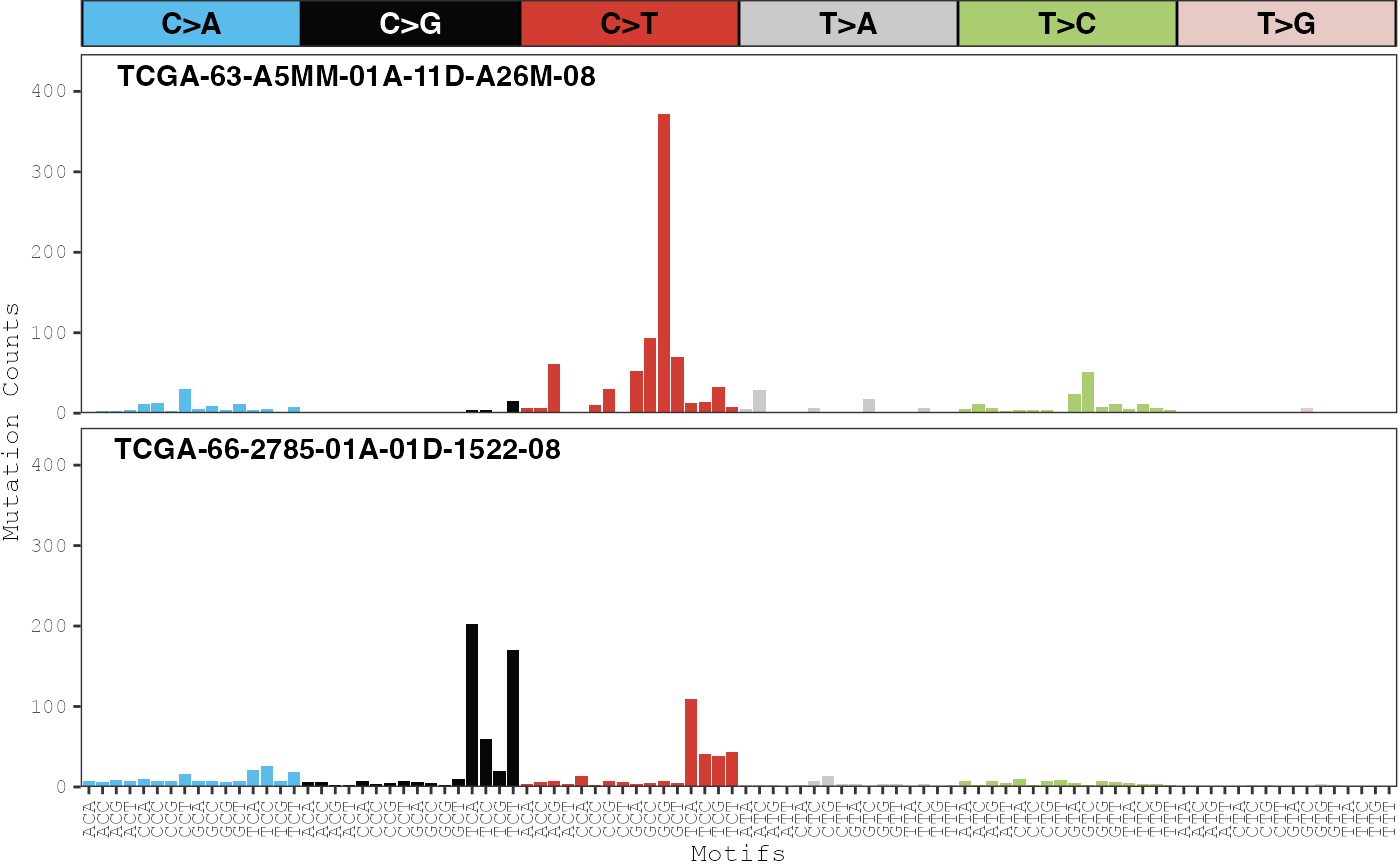

Predict exposures from existing signatures

Predict COSMIC signatures

Instead of discovering mutational signatures and exposures from a dataset de novo, a better result may be obtained by predicting the exposures of signatures that have been previously estimated in other datasets. Predicting exposures for pre-existing signatures may have more sensitivity for detecting active compared to the discovery-based methods as we are incorporating prior information derived from larger datasets. The musicatk package incorporates several methods for estimating exposures given a set of pre-existing signatures. For example, the exposures for COSMIC signatures 1, 4, 7, 13, and 15 can be predicted in our current dataset. Note that we are including COSMIC signature 1 in the prediction even though it did not show up in the discovery algorithm as this signature has been previously shown to be active in lung tumors and we are also including both APOBEC signatures (2 and 13) which were previously combined into 1 signature in the discovery method.

# Load COSMIC V2 data
data("cosmic_v2_sigs")

# Predict pre-existing exposures using the "lda" method
predict_exposure(
  musica = musica_filter, modality = "SBS96",
  signature_res = cosmic_v2_sigs,
  model_id = "result_cosmic_selected_sigs",
  signatures_to_use = c(1, 2, 4, 6, 7, 13), algorithm = "lda"
)

# Plot exposures
plot_exposures(musica_filter, "result_cosmic_selected_sigs", plot_type = "bar",
               num_samples = 50)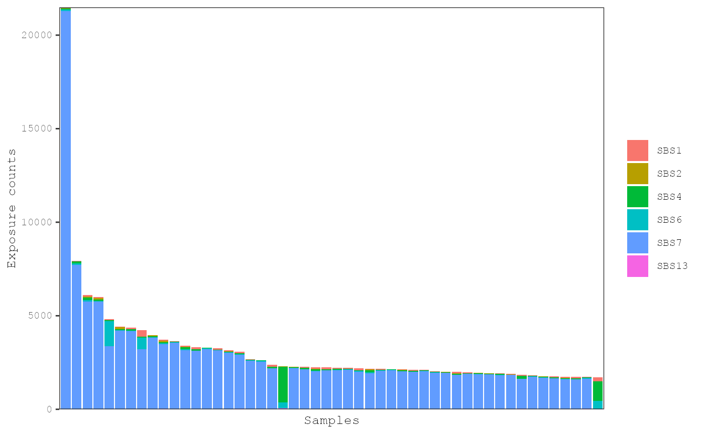

The cosmic_v2_sigs object is just a result_model object containing COSMIC V2 signatures without any sample or exposure information. Note that if signatures_to_use is not supplied by the user, then exposures for all signatures in the result object will be estimated. Any result_model object can be given to the signature_res parameter. Exposures can be predicted for samples in any musica object from any result_model object as long as the same mutation schema was utilized.

Prediction with signature selection

In many cases, researchers will not know the signatures that are active in a cohort of samples beforehand. While it would be easy to predict all COSMIC signatures, this can have detrimental effects on the output. Including signatures not actually active in the cohort of samples may introduce additional noise in the estimates for the exposures for the signatures that are truly present in the dataset. Additionally, including extra signatures may induce a false signal for the exposures of the non-active signatures. The musicatk package has a “two-step” prediction process. In the first step, exposures for all signatures will be estimated. Then a subset of signatures will be selected as “active” in the dataset and only the exposures for the active signatures will be estimated. This two-step process can be done automatically using the auto_predict_grid function:

# Predict exposures with auto selection of signatures
auto_predict_grid(musica_filter, modality = "SBS96",
                  signature_res = cosmic_v2_sigs, algorithm = "lda",
                  model_id = "result_cosmic_auto",
                  sample_annotation = "Tumor_Type")

## LUAD

## LUSC

## SKCM

# See list of selected signatures
rownames(exposures(musica_filter, "result", "SBS96", "result_cosmic_auto"))

##  [1] "SBS1"  "SBS13" "SBS15" "SBS16" "SBS18" "SBS2"  "SBS21" "SBS24" "SBS26"
## [10] "SBS3"  "SBS4"  "SBS6"  "SBS7"

In this result, 13 of the 30 original COSMIC V2 signatures were selected including several signatures that were not previously included in our first prediction with manually selected signatures. If multiple groups of samples are present in the dataset that are expected to have somewhat different sets of active signatures (e.g. multiple tumor types), then this 2-step process can be improved by performing signature selection within each group. This can be achieved by supplying the sample_annoation parameter. In our example, exposures were predicted in the three different tumor types by supplying the Tumor_Type annotation to sample_annotation. This parameter can be left NULL if no grouping annotation is available.

The three major parameters that determine whether a signature is present in a dataset on the first pass are:

min_exists - A signature will be considered active in a sample if its exposure level is above this threshold (Default 0.05).
proportion_samples - A signature will be considered active in a cohort and included in the second pass if it is active in at least this proportion of samples (Default 0.25).
rare_exposure - A signature will be considered active in a cohort and included in the second pass if the proportion of its exposure is above this threshold in at least one sample (Default 0.4). This parameter is meant to capture signatures that produce high number of mutations but are found in a small number of samples (e.g. Mismatch repair).

Assess predicted signatures

It is almost always worthwhile to manually assess and confirm the signatures predicted to be present within a dataset, especially for signatures that have similar profiles to one another. For example, both COSMIC Signature 4 (smoking) and Signature 24 (aflatoxin) were predicted to be present within our dataset. The smoking-related signature is expected as our cohort contains lung cancers, but the aflatoxin signature is unexpected given that it is usually found in liver cancers. These signatures both have a strong concentration of C>A tranversions. In fact, we can see that the predicted exposures for these signatures are highly correlated to each other across samples:

e <- exposures(musica_filter, "result", "SBS96", "result_cosmic_auto")
plot(e["SBS4", ], e["SBS24", ], xlab = "SBS4", ylab = "SBS24")

Therefore, we will want to remove Signature 24 from our final prediction model. Signature 18 is another one with a high prevalence of C>A transversion at specific trinucleotide contexts. However, at least a few samples have high levels of Signature 18 without correspondingly high levels of Signature 4:

plot(e["SBS4", ], e["SBS18", ], xlab = "SBS4", ylab = "SBS18")

plot_exposures(musica_filter, "result_cosmic_auto", num_samples = 25,
               sort_samples = "SBS18")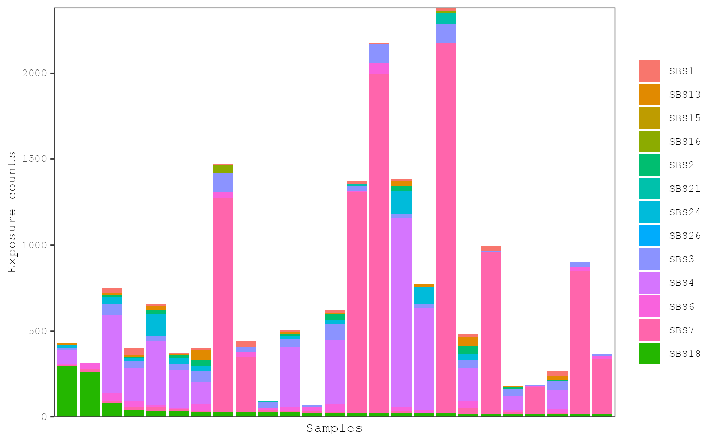

Additionally, 2 of the 3 samples are skin cancers where the smoking signature is not usually expected:

high.sbs18 <- tail(sort(e["SBS18", ]), n = 3)
annot[names(high.sbs18), ]

##                              Tumor_Type ID                            
## TCGA-37-5819-01A-01D-1632-08 "LUSC"     "TCGA-37-5819-01A-01D-1632-08"
## TCGA-EE-A184-06A-11D-A196-08 "SKCM"     "TCGA-EE-A184-06A-11D-A196-08"
## TCGA-22-5472-01A-01D-1632-08 "LUSC"     "TCGA-22-5472-01A-01D-1632-08"

As a final check, we can look at the counts of the individual samples with high levels of Signature 18:

plot_sample_counts(musica_filter, sample_names = "TCGA-ER-A19P-06A-11D-A196-08")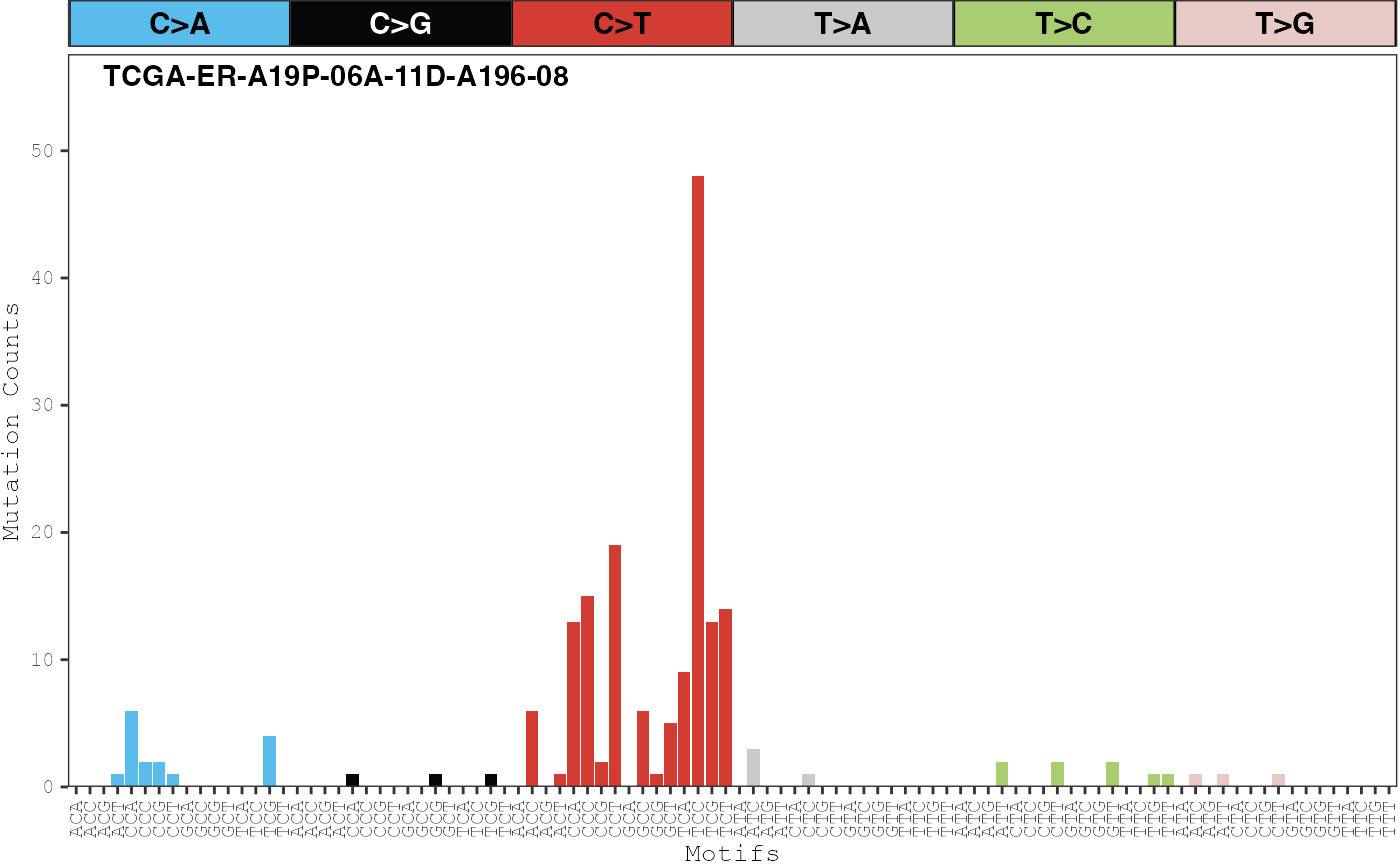

This sample clearly has high levels of both the UV signature confirming that it is likely a skin cancer. Signature 18 is also likely to be active as a high number of C>A mutations at CCA, TCA, and TCT trinucleotide contexts can be observed. Given these results, Signature 18 will be kept in the final analysis.

After additional analysis of other signatures, we also want to remove Signature 3 as that is predominantly found in tumors with BRCA deficiencies (e.g. breast cancer) and in samples with high rates of indels (which are not observed here). The predict_exposure function will be run one last time with the curated list of signatures and this final result will be used in the rest of the down-stream analyses:

# Predict pre-existing exposures with the revised set of selected signatures
predict_exposure(musica = musica_filter, modality = "SBS96",
                 signature_res = cosmic_v2_sigs,
                 signatures_to_use = c(1, 2, 4, 6, 7, 13, 15, 18, 26),
                 model_id = "result_cosmic_final", algorithm = "lda")

Downstream analyses

Visualize relationships between samples with 2-D embedding

The create_umap function embeds samples in 2 dimensions using the umap function from the uwot package. The major parameters for fine tuning the UMAP are n_neighbors, min_dist, and spread. Generally, a higher min_dist will create more separation between the larger groups of samples while a lower See ?uwot::umap for more information on these parameters as well as this tutorial for fine-tuning. Here, a UMAP will be created with standard parameters:

set.seed(1)
create_umap(musica_filter, "result_cosmic_final")

Note that while we are using the result_cosmic_final model which came from the prediction algorithm, we could have also used the ex_result model generated by the discovery algorithm. The plot_umap function will generate a scatter plot of the UMAP coordinates. The points of plot will be colored by the level of a signature by default:

plot_umap(musica_filter, "result_cosmic_final")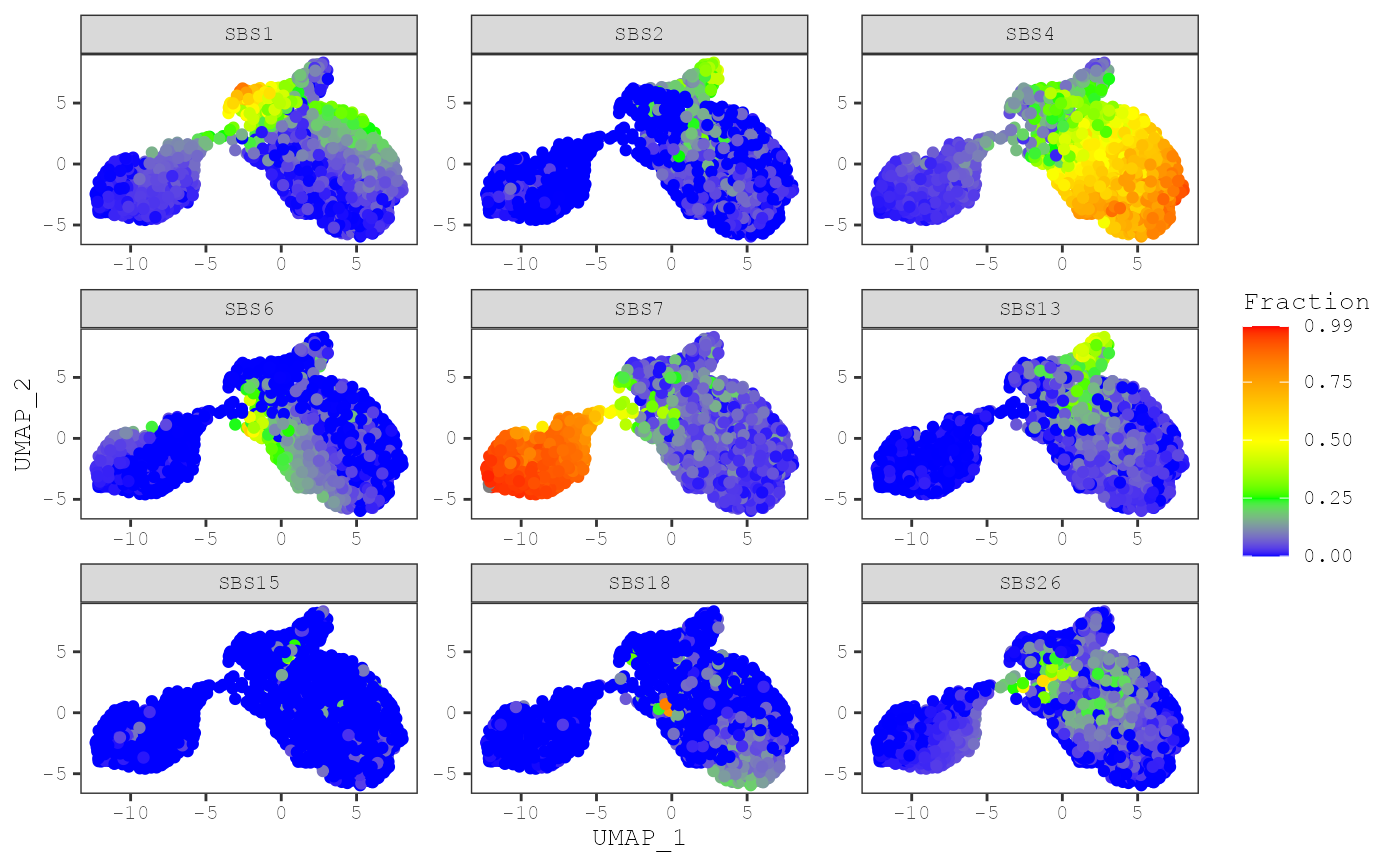

By default, the exposures for each sample will share the same color scale. However, exposures for some signatures may have really high levels compared to others. To make a plot where exposures for each signature will have their own color scale, you can set same_scale = FALSE:

plot_umap(musica_filter, "result_cosmic_final", same_scale = FALSE)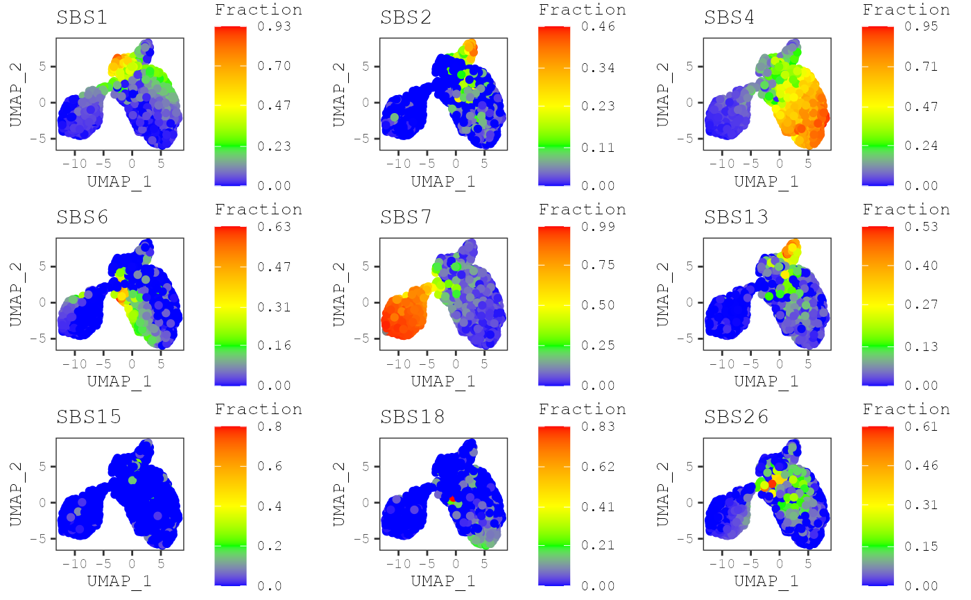

Lastly, points can be colored by a Sample Annotation by setting color_by = "annotation" and the annotation parameter to the name of the annotation:

plot_umap(musica_filter, "result_cosmic_final", color_by = "annotation",
          annotation = "Tumor_Type")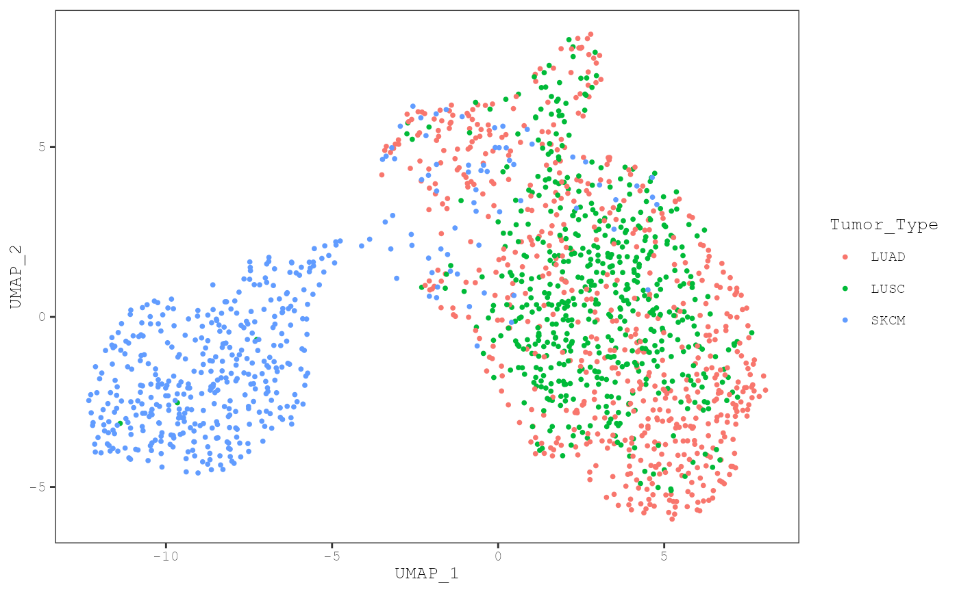

If we set add_annotation_labels = TRUE, the centroid of each group is identified using medians and the labels are plotted at the position of the centroid:

plot_umap(musica_filter, "result_cosmic_final", color_by = "annotation",
          annotation = "Tumor_Type", add_annotation_labels = TRUE)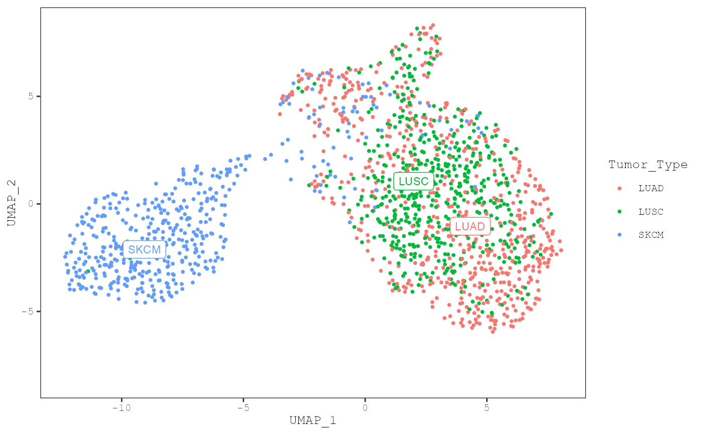

Plotting exposures in a heatmap

Exposures can be displayed in a heatmap where each row corresponds to a siganture and each column correponds to a sample:

plot_heatmap(musica_filter, "result_cosmic_final")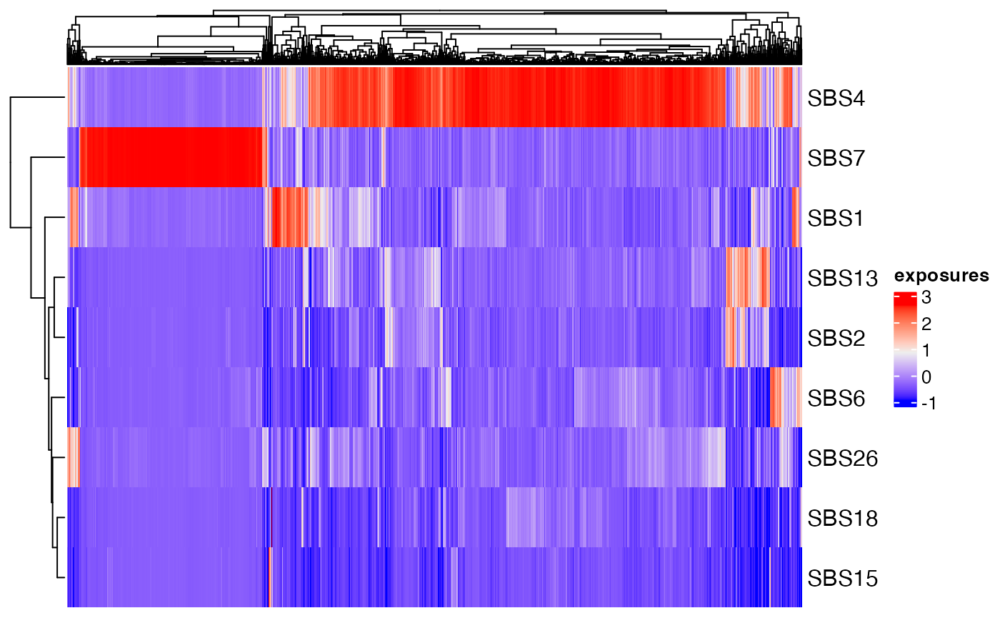

By default, signatures are scaled to have a mean of zero and a standard deviation of 1 across samples (i.e. z-scored). This can be turned off by setting scale = FALSE. Sample annotations can be displayed in the column color bar by setting the annotation parameter:

plot_heatmap(musica_filter, "result_cosmic_final", annotation = "Tumor_Type")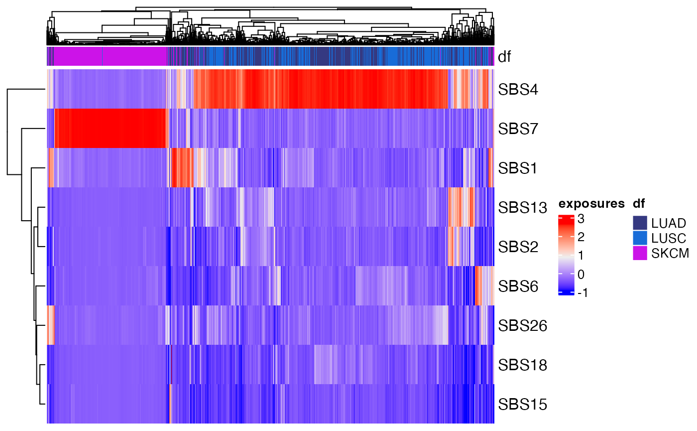

The heatmap shows that Signature 4 and Signature 7 are largely mutually exclusive from one another and can be used to separate lung and skin cancers. Additionally, subsets of signatures or samples can be displayed. For example, if we only want to examine signatures involved in mismatch repair, we can select signatures 6, 15, and 26:

plot_heatmap(musica_filter, "result_cosmic_final", annotation = "Tumor_Type",
             subset_signatures = c("SBS6", "SBS15", "SBS26"))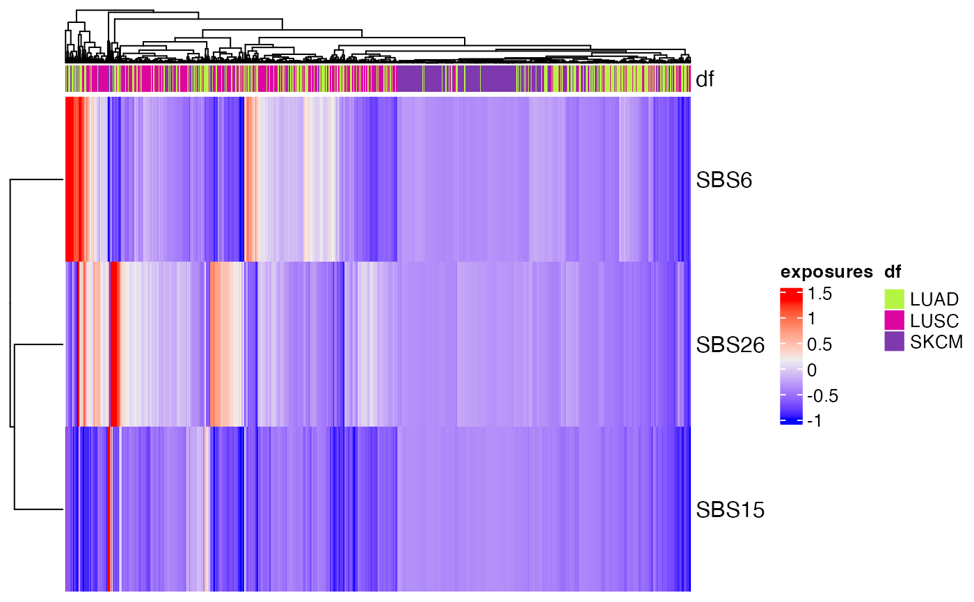

In this heatmap, we can see that only a small subset of distinct samples have relatively higher levels of these signatures.

Clustering samples based on exposures

Samples can be grouped into de novo clusters using a several algorithms from the factoextra and cluster packages such as pam or kmeans. One major challenge is choosing the number of clusters (k). The function k_select has several metrics for examining cluster stability such as total within cluster sum of squares (wss), Silhouette Width (silhouette), and the Gap Statistic (gap_stat).

k_select(musica_filter, "result_cosmic_final", method = "silhouette",
         clust.method = "pam", n = 20)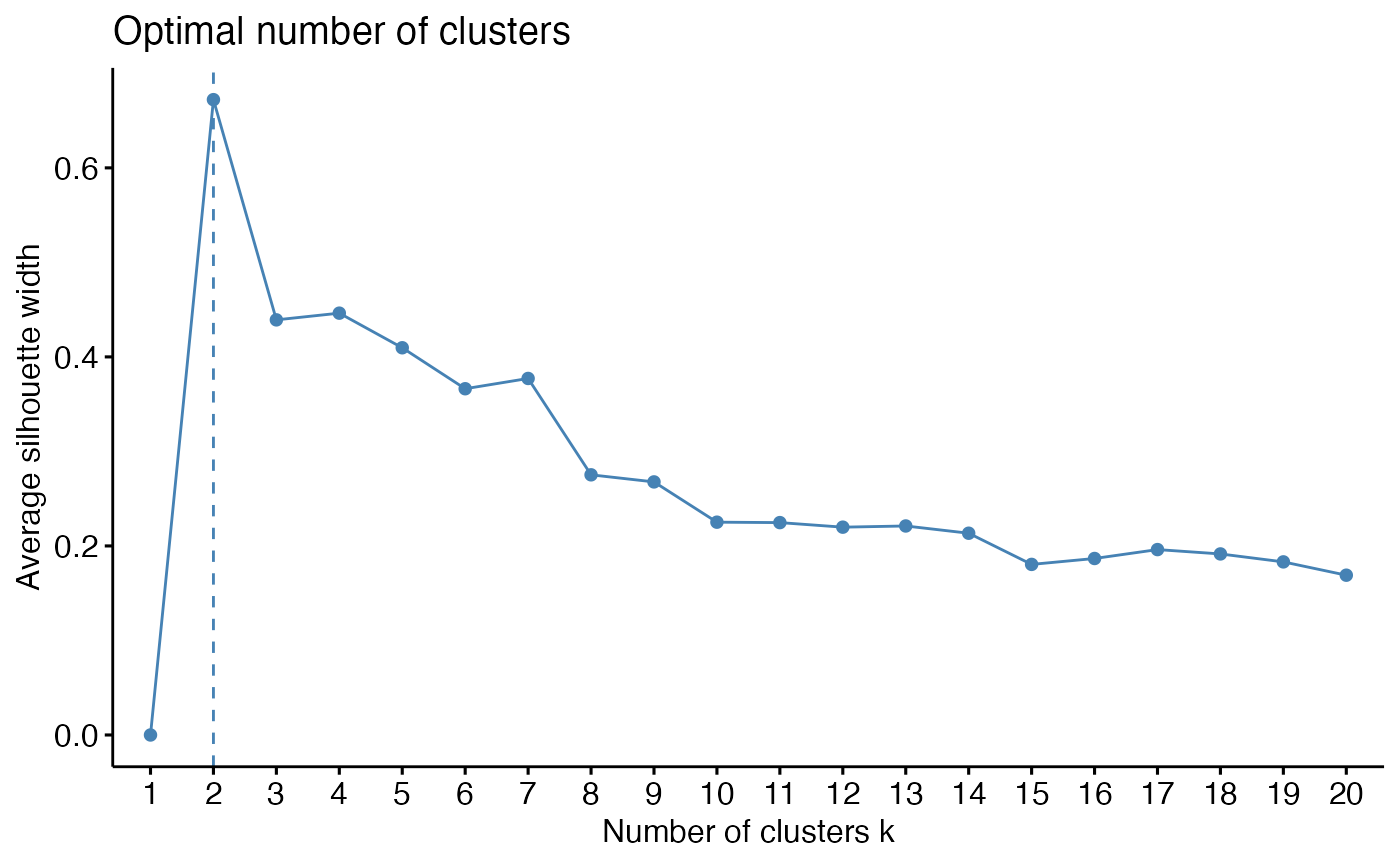

While 2 clusters may be the most optimal choice, this would just correspond to the two large clusters of lung and skin tumors. Therefore, choosing a higher value may be more informative. The next major drop in the silhouette width is after k = 6, so we will select this moving forward and perform the clustering:

clusters <- cluster_exposure(musica_filter, "result_cosmic_final",
                             method = "pam", nclust = 6)

## Metric: 'euclidean'; comparing: 1614 vectors.

Clusters can be visualized on the UMAP with the plot_cluster function:

clusters[, 1] <- as.factor(clusters[, 1])
plot_cluster(musica_filter, "result_cosmic_final", cluster = clusters,
             group = "none")

Additional features

Plotly for interactive plots

The functions plot_signatures, plot_exposures, and plot_umap have the ability to create ggplotly plots by simply specifying plotly = TRUE. Plotly plots are interactive and allow users to zoom and re-sizing plots, turn on and off annotation types and legend values, and hover over elements of the plots (e.g. bars or points) to more information about that element (e.g. sample name). Here are examples of plot_signatures and plot_exposures

plot_signatures(musica_filter, "result_cosmic_final", plotly = TRUE)

plot_exposures(musica_filter, "result_cosmic_final", num_samples = 25,
               plotly = TRUE)

COSMIC signatures annotated to be active in a tumor type

The signatures predicted to be present in each tumor type according to the COSMIC V2 database can be quickly retrieved. For example, we can find which signatures are predicted to be present in lung cancers:

cosmic_v2_subtype_map("lung")

## lung adeno

## 124561317

## lung  small cell

## 14515

## lung  squamous

## 124513

Creating custom tables

Custom count tables can be created from user-defined mutation-level annotations using the build_custom_table function.

# Adds strand information to the 'variant' table
annotate_transcript_strand(musica, genome_build = "hg38", build_table = FALSE)

##   2135 genes were dropped because they have exons located on both strands
##   of the same reference sequence or on more than one reference sequence,
##   so cannot be represented by a single genomic range.
##   Use 'single.strand.genes.only=FALSE' to get all the genes in a
##   GRangesList object, or use suppressMessages() to suppress this message.

# Generates a count table from strand
build_custom_table(
  musica = musica, variant_annotation = "Transcript_Strand",
  name = "Transcript_Strand",
  description = "A table of transcript strand of variants",
  data_factor = c("T", "U"), overwrite = TRUE
)

Session Information

sessionInfo()

## R version 4.4.0 (2024-04-24)
## Platform: aarch64-apple-darwin20
## Running under: macOS Ventura 13.1
## 
## Matrix products: default
## BLAS:   /Library/Frameworks/R.framework/Versions/4.4-arm64/Resources/lib/libRblas.0.dylib 
## LAPACK: /Library/Frameworks/R.framework/Versions/4.4-arm64/Resources/lib/libRlapack.dylib;  LAPACK version 3.12.0
## 
## locale:
## [1] en_US.UTF-8/en_US.UTF-8/en_US.UTF-8/C/en_US.UTF-8/en_US.UTF-8
## 
## time zone: America/New_York
## tzcode source: internal
## 
## attached base packages:
## [1] stats     graphics  grDevices datasets  utils     methods   base     
## 
## other attached packages:
## [1] TCGAbiolinks_2.32.0 musicatk_2.0.0      NMF_0.27           
## [4] Biobase_2.64.0      BiocGenerics_0.50.0 cluster_2.1.6      
## [7] rngtools_1.5.2      registry_0.5-1     
## 
## loaded via a namespace (and not attached):
##   [1] RcppAnnoy_0.0.22                        
##   [2] BiocIO_1.14.0                           
##   [3] bitops_1.0-7                            
##   [4] filelock_1.0.3                          
##   [5] matrixTests_0.2.3                       
##   [6] tibble_3.2.1                            
##   [7] R.oo_1.26.0                             
##   [8] XML_3.99-0.17                           
##   [9] factoextra_1.0.7                        
##  [10] lifecycle_1.0.4                         
##  [11] httr2_1.0.2                             
##  [12] rstatix_0.7.2                           
##  [13] doParallel_1.0.17                       
##  [14] NLP_0.2-1                               
##  [15] lattice_0.22-6                          
##  [16] vroom_1.6.5                             
##  [17] MASS_7.3-61                             
##  [18] crosstalk_1.2.1                         
##  [19] backports_1.5.0                         
##  [20] magrittr_2.0.3                          
##  [21] plotly_4.10.4                           
##  [22] sass_0.4.9                              
##  [23] rmarkdown_2.27                          
##  [24] jquerylib_0.1.4                         
##  [25] yaml_2.3.9                              
##  [26] BSgenome.Hsapiens.UCSC.hg38_1.4.5       
##  [27] topicmodels_0.2-16                      
##  [28] cowplot_1.1.3                           
##  [29] DBI_1.2.3                               
##  [30] RColorBrewer_1.1-3                      
##  [31] abind_1.4-5                             
##  [32] zlibbioc_1.50.0                         
##  [33] rvest_1.0.4                             
##  [34] GenomicRanges_1.56.1                    
##  [35] purrr_1.0.2                             
##  [36] R.utils_2.12.3                          
##  [37] RCurl_1.98-1.16                         
##  [38] VariantAnnotation_1.50.0                
##  [39] rappdirs_0.3.3                          
##  [40] circlize_0.4.16                         
##  [41] GenomeInfoDbData_1.2.12                 
##  [42] IRanges_2.38.1                          
##  [43] S4Vectors_0.42.1                        
##  [44] ggrepel_0.9.5                           
##  [45] tm_0.7-13                               
##  [46] irlba_2.3.5.1                           
##  [47] BiocStyle_2.32.1                        
##  [48] conclust_1.1                            
##  [49] pkgdown_2.1.0                           
##  [50] codetools_0.2-20                        
##  [51] DelayedArray_0.30.1                     
##  [52] xml2_1.3.6                              
##  [53] tidyselect_1.2.1                        
##  [54] shape_1.4.6.1                           
##  [55] UCSC.utils_1.0.0                        
##  [56] farver_2.1.2                            
##  [57] TCGAbiolinksGUI.data_1.24.0             
##  [58] matrixStats_1.3.0                       
##  [59] stats4_4.4.0                            
##  [60] BiocFileCache_2.12.0                    
##  [61] GenomicAlignments_1.40.0                
##  [62] jsonlite_1.8.8                          
##  [63] GetoptLong_1.0.5                        
##  [64] iterators_1.0.14                        
##  [65] systemfonts_1.1.0                       
##  [66] foreach_1.5.2                           
##  [67] tools_4.4.0                             
##  [68] progress_1.2.3                          
##  [69] TxDb.Hsapiens.UCSC.hg19.knownGene_3.2.2 
##  [70] ragg_1.3.2                              
##  [71] Rcpp_1.0.12                             
##  [72] glue_1.7.0                              
##  [73] gridExtra_2.3                           
##  [74] SparseArray_1.4.8                       
##  [75] xfun_0.45                               
##  [76] MatrixGenerics_1.16.0                   
##  [77] GenomeInfoDb_1.40.1                     
##  [78] dplyr_1.1.4                             
##  [79] withr_3.0.1                             
##  [80] combinat_0.0-8                          
##  [81] BiocManager_1.30.23                     
##  [82] fastmap_1.2.0                           
##  [83] MCMCprecision_0.4.0                     
##  [84] fansi_1.0.6                             
##  [85] digest_0.6.36                           
##  [86] R6_2.5.1                                
##  [87] textshaping_0.4.0                       
##  [88] colorspace_2.1-0                        
##  [89] gtools_3.9.5                            
##  [90] biomaRt_2.60.1                          
##  [91] RSQLite_2.3.7                           
##  [92] R.methodsS3_1.8.2                       
##  [93] utf8_1.2.4                              
##  [94] tidyr_1.3.1                             
##  [95] generics_0.1.3                          
##  [96] renv_1.0.7                              
##  [97] data.table_1.15.4                       
##  [98] rtracklayer_1.64.0                      
##  [99] prettyunits_1.2.0                       
## [100] httr_1.4.7                              
## [101] htmlwidgets_1.6.4                       
## [102] S4Arrays_1.4.1                          
## [103] uwot_0.2.2                              
## [104] pkgconfig_2.0.3                         
## [105] gtable_0.3.5                            
## [106] modeltools_0.2-23                       
## [107] blob_1.2.4                              
## [108] ComplexHeatmap_2.20.0                   
## [109] XVector_0.44.0                          
## [110] htmltools_0.5.8.1                       
## [111] carData_3.0-5                           
## [112] clue_0.3-65                             
## [113] scales_1.3.0                            
## [114] tidyverse_2.0.0                         
## [115] TxDb.Hsapiens.UCSC.hg38.knownGene_3.18.0
## [116] png_0.1-8                               
## [117] knitr_1.48                              
## [118] rstudioapi_0.16.0                       
## [119] tzdb_0.4.0                              
## [120] reshape2_1.4.4                          
## [121] rjson_0.2.21                            
## [122] curl_5.2.1                              
## [123] cachem_1.1.0                            
## [124] GlobalOptions_0.1.2                     
## [125] stringr_1.5.1                           
## [126] parallel_4.4.0                          
## [127] AnnotationDbi_1.66.0                    
## [128] restfulr_0.0.15                         
## [129] desc_1.4.3                              
## [130] pillar_1.9.0                            
## [131] grid_4.4.0                              
## [132] vctrs_0.6.5                             
## [133] slam_0.1-50                             
## [134] ggpubr_0.6.0                            
## [135] car_3.1-2                               
## [136] dbplyr_2.5.0                            
## [137] evaluate_0.24.0                         
## [138] readr_2.1.5                             
## [139] GenomicFeatures_1.56.0                  
## [140] cli_3.6.3                               
## [141] compiler_4.4.0                          
## [142] Rsamtools_2.20.0                        
## [143] rlang_1.1.4                             
## [144] crayon_1.5.3                            
## [145] ggsignif_0.6.4                          
## [146] labeling_0.4.3                          
## [147] plyr_1.8.9                              
## [148] fs_1.6.4                                
## [149] stringi_1.8.4                           
## [150] viridisLite_0.4.2                       
## [151] philentropy_0.8.0                       
## [152] gridBase_0.4-7                          
## [153] BiocParallel_1.38.0                     
## [154] munsell_0.5.1                           
## [155] Biostrings_2.72.1                       
## [156] lazyeval_0.2.2                          
## [157] Matrix_1.7-0                            
## [158] BSgenome_1.72.0                         
## [159] hms_1.1.3                               
## [160] bit64_4.0.5                             
## [161] ggplot2_3.5.1                           
## [162] KEGGREST_1.44.1                         
## [163] SummarizedExperiment_1.34.0             
## [164] highr_0.11                              
## [165] broom_1.0.6                             
## [166] memoise_2.0.1                           
## [167] bslib_0.7.0                             
## [168] bit_4.0.5                               
## [169] downloader_0.4

Aaron Chevalier, Joshua Campbell

Compiled December 16, 2024