Introduction
This section comes together with the previous section Differential Expression. The basic strategy singleCellTK (SCTK) uses to find biomarkers is to iteratively identify the significantly up-regulated features of each group of cells against all the other cells. This means, the function we have (runFindMarker()) is a wrapper of functions that do differential expression (DE) analysis, which would be invoked in a loop. For the detail of the DE functions and DE computation methods, please refer to the Differential Expression documentation.
To view detailed instructions on how to use these methods, please select ‘Interactive Analysis’ for shiny application or ‘Console Analysis’ for using these methods on R console from the tabs below:
Workflow Guide
Entry of The Panel
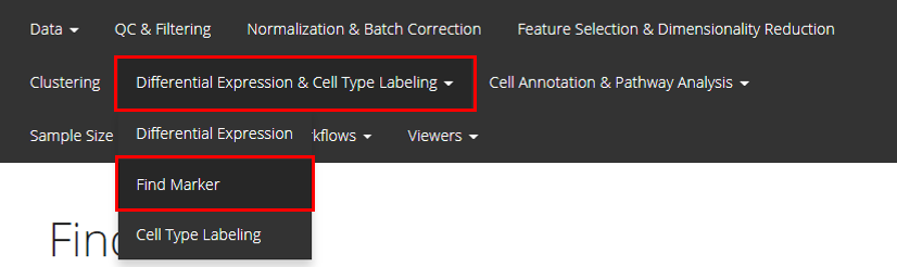
From anywhere of the UI, the panel for marker finding can be accessed from the top navigation panel at the circled tab shown below.
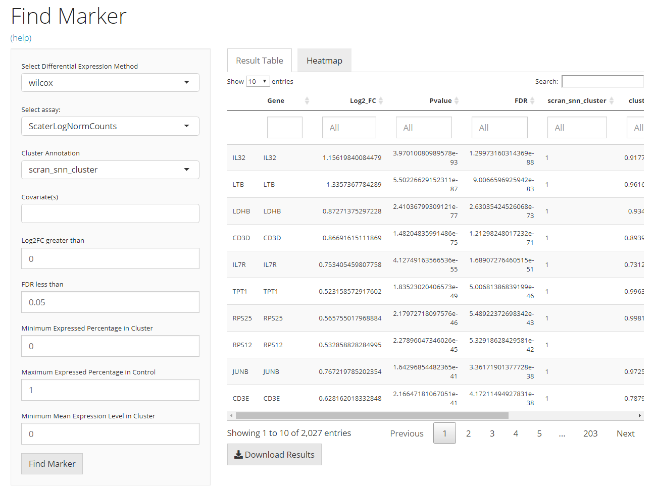
The UI is constructed in a sidebar pattern. The sidebar on the left is mainly for the parameters essential for running the marker finding algorithm. The main panel on the right is for demonstrating the results, including the marker table and the heatmap visualization.
Detail: Algorithm Parameters
- Method selection - selection input “Select Differential Expression Method”. Users will choose which method to use. The method here means the intrinsic dependency used for differential expression (DE) analysis.
- Assay selection - selection input “Select Assay”. Users will choose which expression data matrix to use for marker detection. Note that for method “MAST” and “Limma”, a log-normalized feature expression matrix is required.
- Cluster definition - selection input “Cluster Annotation”. Users will choose a cell level annotation, which defines the cluster assignment for each cell.
- Covariate selection - selection input “Covariate(s)”. A covariate is another set of categorization on the cells involved in the analysis, used for modeling. Multiple selections are acceptable.
- Log2FC cutoff setting - numeric input “Log2FC greater than”. The cutoff set here will rule out DE genes with absolute value of Log2FC (logged fold change) smaller than the cutoff from the result.
- FDR cutoff setting - numeric input “FDR less than”. The cutoff set here will rule out DE genes with FDR (false discovery rate) value more than the cutoff from the result.
- Expression percentage cutoff - numeric inputs “Minimum Expressed Percentage in Cluster” and “Maximum Expressed Percentage in Control”. These are filters that will be applied on the result table. Known that the markers for one cluster is identified by performing DE analysis on this cluster against all other cells, the first parameter rules out the marker genes that are expressed in less than a percentage of cells in the cluster of interests. In a similar way, the second parameter excludes the marker genes expressed in more that a percentage of cells in all other clusters.
- Mean expression level cutoff - numeric input “Minimum Mean Expression Level in Cluster”. Following the last bullet point, this parameter will keep only the marker genes with mean expression level in the cluster higher than higher than a value.
Main Panel - Result Table
The table is shown in the figure above. In this tab, there will be a table for all the markers detected and passed the filters. It is constructed with 5 columns, including “Gene” - the default feature identifiers (not necessarily a gene ID or symbol, depending on the background SCE object); “Log2_FC”, “Pvalue” and “FDR” - the statistics that supports the detection; and the fifth one that labels which cluster the marker is for, and the column name is exactly the “cluster annotation” selected in the sidebar. Users can also download the table in comma-separated value (CSV) format, by clicking “Download Result Table” button.
Main Panel - Heatmap
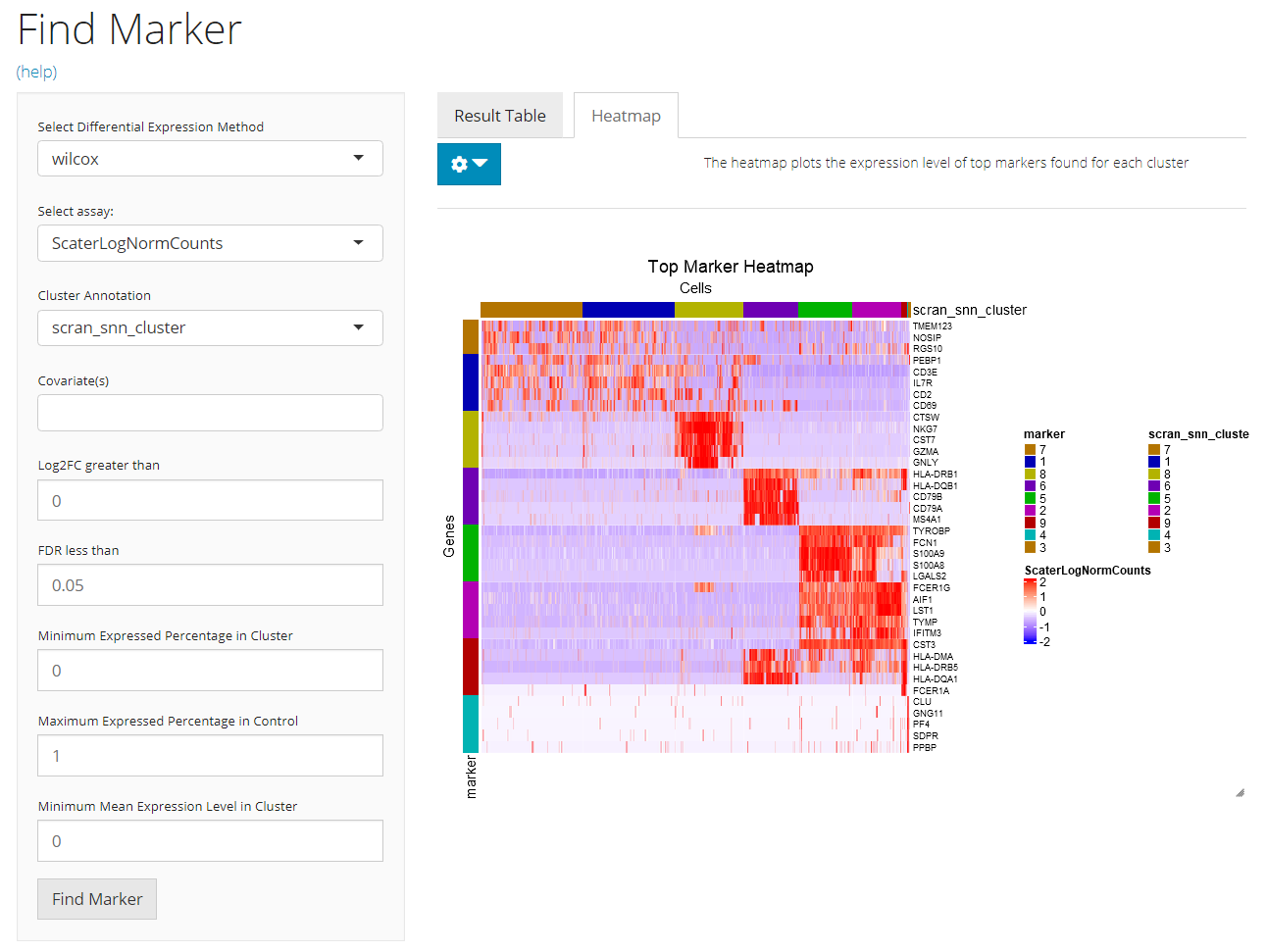
A heatmap will be automatically generated after running the marker detection process. Users can tweak the options for plotting by clicking on the blue clog button on the top-left.
Detail: Heatmap Plotting Options
- Cluster ordering - radio button “Order blocks by”. User will determine here whether to order the columns of the heatmap by the cluster name (i.e. annotation) or the size (i.e. number of cells). Checkbox “Decreasing”. Users can check this option for putting the alphabetically latter cluster or cluster with the largest size on the left.
- Top N marker cutoff - checkbox and numeric input “Plot Top N markers of each cluster”. If the checkbox is not checked, all markers passing the running filter (mentioned above) and plotting filters (will mention below) will be plotted. Otherwise checked, only the top
Nmarkers, asNis the input numeric value in the numeric input below the checkbox, for each cluster will be plotted. The ranking is based on Log2FC value. When less thanNmarkers are detected for one cluster, all of them will be plotted. - Log2FC cutoff - numeric input “Plot Log2FC greater than”. The cutoff set here will rule out markers with absolute value of Log2FC (logged fold change) smaller than the cutoff from the plotting. This will not affect the result saved when running the algorithm.
- FDR cutoff - numeric input "". The cutoff set here will rule out markers with FDR (false discovery rate) value more than the cutoff from the plotting. Similarly, this will not affect the result saved when running the algorithm.
- Expression percentage cutoff - numeric inputs “Plot Cluster Expression Percentage More Than” and “Plot Control Expression Percentage Less Than”. These are filters that will be applied on the result table. Known that the markers for one cluster is identified by performing DE analysis on this cluster against all other cells, the first parameter rules out the marker genes that are expressed in less than a percentage of cells in the cluster of interests. In a similar way, the second parameter excludes the marker genes expressed in more that a percentage of cells in all other clusters.
- Mean expression level cutoff - numeric input “Plot Mean Cluster Expression Level More Than”. Following the last bullet point, this parameter will keep only the marker genes with mean expression level in the cluster higher than higher than a value.
- Additional annotation - multiple selection input “Additional feature annotation” and “Additional cell annotation”. User can add up more cell or gene annotation to the heatmap legend.
Parameters
As per SCTK’s strategy, the primary input is limited to an SingleCellExperiment (SCE) object, which has been through preprocessing steps with cluster labels annotated. While the iteration is a fixed pattern, the parameters needed are rather simple:
sce <- runFindMarker(inSCE = sce, useAssay = "logcounts", cluster = "cluster", covariates = NULL, log2fcThreshold = 0.25, fdrThreshold = 0.05)Here all arguments execpt the input SCE object (inSCE) are set by default. method can only be chosen from the table above. cluster and covariates should be given a single string which is present in names(colData(inSCE)). cluster is required for grouping cells, while covariates is optional for DE detection. log2fcThreshold and fdrThreshold are numeric and has to be set in plausible range. log2fcThrshold has to be positive and fdrThreshold has to be greater than zero and less than one.
The returned SCE object will contain the updated information of the markers identified in its metadata slot.
Example
Preprocessing
The preprocessing for obtaining cluster assignment was done using the exactly same workflow presented in the A La Carte Workflow Tutorial.
library(singleCellTK)
sce <- importExampleData("pbmc3k")
sce <- runPerCellQC(sce, mitoRef = "human", mitoIDType = "symbol", mitoGeneLocation = "rownames")
sce <- subsetSCECols(sce, colData = c('total > 600', 'detected > 300', 'mito_percent < 5'))
sce <- scaterlogNormCounts(sce, useAssay = "counts", assayName = "logcounts")
sce <- runModelGeneVar(sce, useAssay = "logcounts")
sce <- setTopHVG(sce, method = "modelGeneVar")
sce <- scaterPCA(inSCE = sce, useAssay = "logcounts", useFeatureSubset = "HVG_modelGeneVar2000",
                 reducedDimName = "PCA", seed = 12345)
sce <- runScranSNN(sce, useReducedDim = "PCA", nComp = 10, k = 14,
                   weightType = "jaccard", clusterName = "cluster", seed = 12345)
sce <- runUMAP(sce, useReducedDim = "PCA", initialDims = 10, reducedDimName = "UMAP", seed = 12345)
And we can visualize the cell populations on the UMAP with cluster labeled.
plotSCEDimReduceColData(sce, colorBy = "cluster", reducedDimName = "UMAP")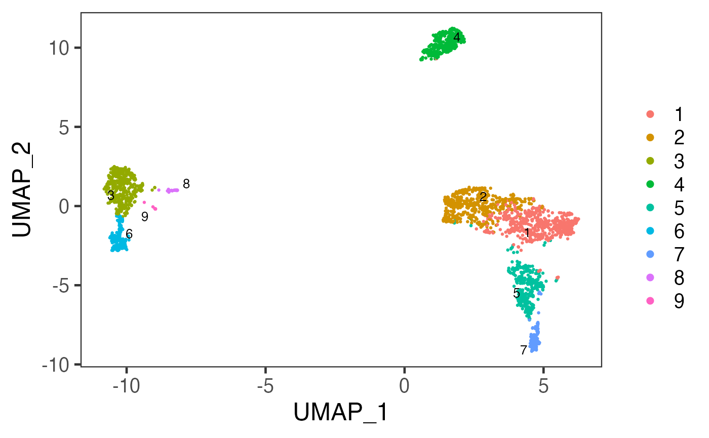
Get Markers
Then we call runFindMarker() on the clustered data, with the cluster annotation just obtained, "cluster".
sce <- runFindMarker(inSCE = sce, useAssay = "logcounts", cluster = "cluster")Results
After successfully running runFindMarker(), the result marker table would be stored in metadata(sce). This table can be fetched by getFindMarkerTopTable(). Argument topN controls how many top markers, that pass filters, to include for each clsuter.
getFindMarkerTopTable(sce, log2fcThreshold = 0, minClustExprPerc = 0.5, topN = 1)## Gene Log2_FC Pvalue FDR cluster clusterExprPerc
## 8764 IL7R 0.8117772 9.627633e-63 5.253157e-59 1 0.7500000
## 309761 NOSIP 0.5887454 1.941718e-38 6.553399e-36 2 0.6821561
## 1956 S100A9 4.3853548 2.397248e-207 3.924055e-203 3 0.9977064
## 30657 CD79A 2.2532545 1.452148e-151 1.188511e-147 4 0.9257143
## 26825 CCL5 3.0924934 1.691729e-148 5.538382e-144 5 0.9712644
## 106091 LST1 2.8683989 1.038405e-98 1.133177e-94 6 1.0000000
## 310761 NKG7 4.2398710 3.256027e-82 1.065958e-77 7 1.0000000
## 288182 CST3 3.2975861 2.221917e-16 1.039159e-12 8 1.0000000
## 7697 PPBP 5.9620589 9.423341e-07 2.504757e-03 9 1.0000000
## ControlExprPerc clusterAveExpr
## 8764 0.31156265 1.266208
## 309761 0.36716132 1.069871
## 1956 0.23094477 4.733569
## 30657 0.04172156 2.296094
## 26825 0.21676174 3.470436
## 106091 0.30477759 3.454109
## 310761 0.25687702 4.781861
## 288182 0.39113680 4.371755
## 7697 0.02406417 5.989445Similarly to the Differential Expression section, we also provide a automated and organized heatmap plotting for the markers:
plotFindMarkerHeatmap(sce, log2fcThreshold = 0, minClustExprPerc = 0.5, maxCtrlExprPerc = 0.5, rowLabel = TRUE)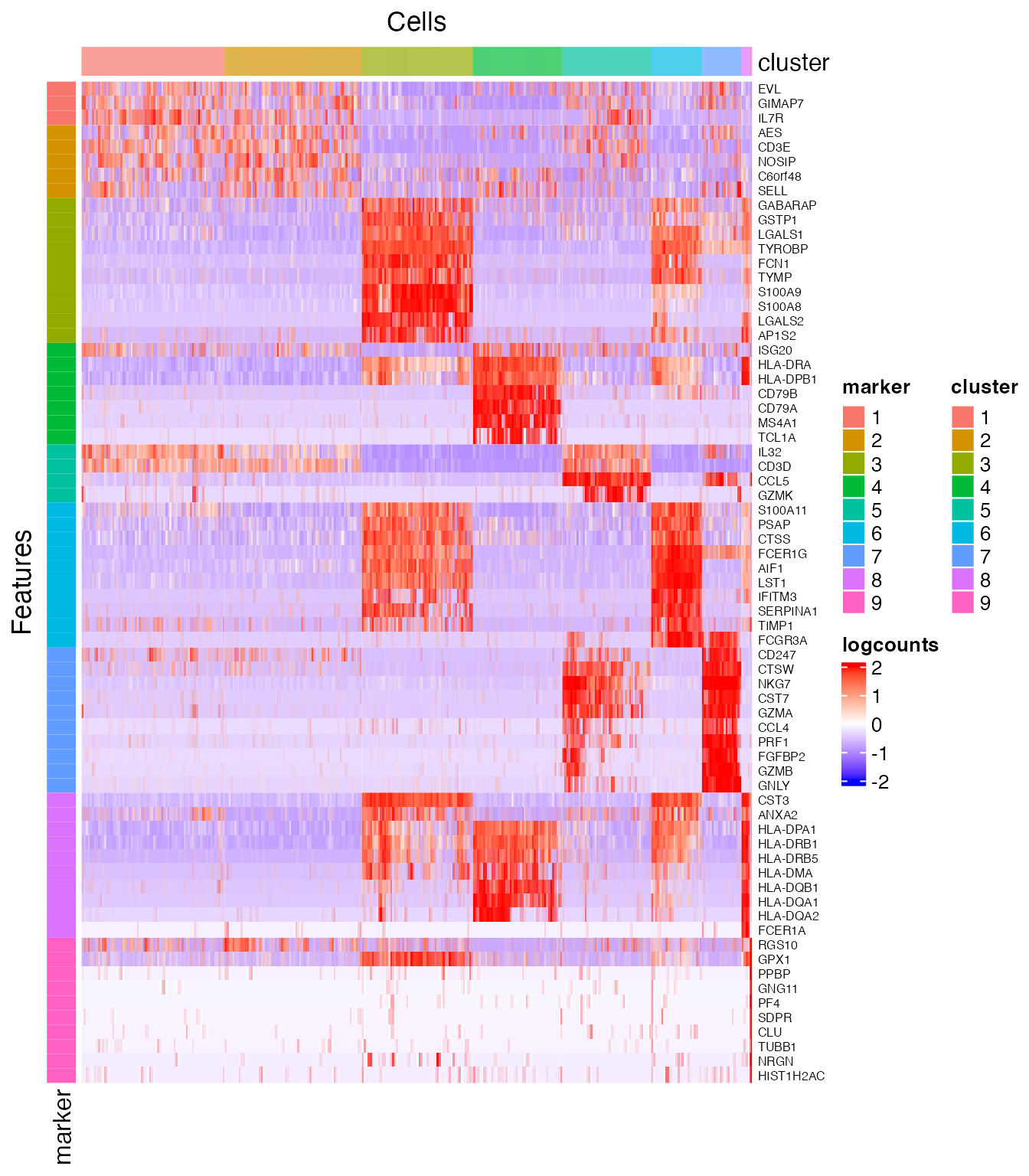
Note that when plotting the heatmap, the genes that are identified as up-regulated in multiple clusters will be considered only for the one cluster with the highest fold-change, while all of them are still kept in the table in metadata.