Batch Correction on SingleCellExperiment Object

Introduction

For this section, we wrapped 12 methods into functions that perform batch effect correction on an SingleCellExperiment (SCE) object and return the input SCE object with a corrected matrix updated in-place.

Here is a table for the method names, citations, corresponding wrapper functions and where the results are updated:

Method	Citation	Function	Result Slots
BBKNN	Polański, Krzysztof and et al., 2019	runBBKNN()	`reducedDim`
ComBat	Yuqing Zhang and et al., 2018	runComBat()	`assay`
FastMNN	Aaron Lun, 2018	runFastMNN()	`reducedDim`
MNN	Laleh Haghverdi, 2018	runMNNCorrect()	`assay`
Harmony	Ilya Korsunsky and et al., 2019	runHarmony()	`reducedDim`
LIGER	Joshua Welch, et al., 2018	runLIGER()	`reducedDim`
Limma	Gordon K Smyth, et al., 2003	runLimmaBC()	`assay`
Scanorama	Brian Hie et al, 2019	runSCANORAMA()	`assay`
scGen	Mohammad Lotfollah et al., 2019	runSCGEN()	`assay`
scMerge	Yingxin Lin et al., 2019	runSCMerge()	`assay`
Seurat Integration	Tim Stuart et al., 2019	runSeurat3Integration()	`altExp`
ZINBWaVE	Davide Risso et al., 2018	runZINBWaVE()	`reducedDim`

For a result returned in reducedDim, it means that some sorts of dimension reduction method, such as PCA and UMAP, is performed during the correction. For a result returned in assay, all of the original features (i.e. genes) remain the same, thus it is a full-sized assay. For a result returned in altExp, it means that the values in the corrected assay still stand for the expression level of the original features, instead of any low-dimension embedding, but the number of these features are less than original due to potential subsetting steps in the calculation.

Additional Required Dependencies

SCTK provides options of “BBKNN” and “Scanorama” for batch correction. These methods are Python based. In order to successfully apply these methods, users have to get a Python3 environment activated and indentifiable for R-reticulate. For users convenience, SCTK provides one-click functions to install the environment together with the libraries. These functions will by default also install the Python libraries used for Quality Control.

sctkPythonInstallConda()
# OR
sctkPythonInstallVirtualEnv()

Running the pipeline

To run the pipeline, the most basic requirements are:

An assay of expression value, usually pre-processed.
The annotation of the batches.

As we adopt SingleCellExperiment (sce) object through out the whole SCTK for a collection of all matrices and metadatas of the dataset of interests, the assay to be corrected, called "assayToCorr", has to be saved at assay(sce, "assayToCorr"). Meanwhile, the batch annotation information has to be saved in a column of colData(sce).

Note that the batch annotation should better be saved as a factor in the colData, especially when the batches are represented by integer numbers, because some downstream analysis are likely to parse the non-character and non-logical information as continuous values instead of categorical values.

Command line example

Prepare an SCE object with multiple batches

Here we present an example dataset that is combined from “pbmc3k” and “pbmc4k” (Kasper D. Hansen et al., 2017), which you can import by a function called importExampleData().

library(singleCellTK)
pbmc6k <- importExampleData('pbmc6k')
pbmc8k <- importExampleData('pbmc8k')
print(paste(dim(pbmc6k), c('genes', 'cells')))
print(paste(dim(pbmc8k), c('genes', 'cells')))

## [1] "32738 genes" "5419 cells" 
## [1] "33694 genes" "8381 cells"

There is a function called combineSCE(), which accepts a list of SCE objects as input and returns a combined SCE object. This function requires that the number of genes in each SCE object has to be the same, and the gene metadata (i.e. rowData) has to match with each other if the same fields exist. Therefore, we need some pre-process for the combination. Users do not necessarily have to follow the same way, depending on how the raw datasets are provided.

## Combine the two SCE objects
sce.combine <- combineSCE(sceList = list(pbmc6k = pbmc6k, pbmc8k = pbmc8k), 
                          by.r = names(rowData(pbmc6k)), 
                          by.c = names(colData(pbmc6k)), 
                          combined = TRUE)
table(sce.combine$sample)

## 
## pbmc6k pbmc8k 
##   5419   8381

In this manual, we only present a toy example instead of a best practice for real data. Therefore, QC and filtering are skipped.
Additionally, most of the batch correction methods provided require a log-normalized assay as input, users can check the required assay type of each method by looking at its default setting. (i.e. if by default useAssay = "logcounts", then it requires log-normalized assay; else if by default useAssay = "counts", then the raw count assay.)

## Simply filter out the genes that are expressed in less than 1% of all cells.
sce.filter <- sce.combine[rowSums(assay(sce.combine) > 0) >= 0.01 * ncol(sce.combine),]
sce.filter

## class: SingleCellExperiment 
## dim: 10415 13800 
## metadata(0):
## assays(1): counts
## rownames(10415): AP006222.2 RP11-206L10.9 ... URB1-AS1 AC007325.4
## rowData names(4): rownames ENSEMBL_ID Symbol_TENx Symbol
## colnames(13800): pbmc6k_AAACATACAACCAC-1 pbmc6k_AAACATACACCAGT-1 ...
##   pbmc8k_TTTGTCATCTCGAGTA-1 pbmc8k_TTTGTCATCTGCTTGC-1
## colData names(13): rownames Sample ... Date_published sample
## reducedDimNames(0):
## altExpNames(0):

sce.small <- sce.filter[sample(nrow(sce.filter), 800), sample(ncol(sce.filter), 800)]
sce.small <- scaterlogNormCounts(inSCE = sce.small,
                                 useAssay = 'counts',
                                 assayName = 'logcounts')
sce.small

## class: SingleCellExperiment 
## dim: 800 800 
## metadata(1): assayType
## assays(2): counts logcounts
## rownames(800): MTURN DLD ... SIT1 PIP4K2A
## rowData names(4): rownames ENSEMBL_ID Symbol_TENx Symbol
## colnames(800): pbmc8k_GCGCAGTAGTCCGGTC-1 pbmc8k_AACCATGTCTCGTATT-1 ...
##   pbmc8k_GCTTGAAGTTTAAGCC-1 pbmc8k_GAGTCCGGTATATCCG-1
## colData names(14): rownames Sample ... sample sizeFactor
## reducedDimNames(0):
## altExpNames(0):

Run a batch correction method on the prepared SCE object

The basic way to run a batch correction method from SingleCellTK is to select a function for the corresponding method, input the SCE object, specify the assay to correct, and the batch annotation.

For example, here we will try the batch correction method provided by Limma, which fits a linear model to the data.

sce.small <- runLimmaBC(inSCE = sce.small, 
                        useAssay = 'logcounts', 
                        batch = 'sample', 
                        assayName = 'LIMMA')
sce.small

## class: SingleCellExperiment 
## dim: 800 800 
## metadata(1): assayType
## assays(3): counts logcounts LIMMA
## rownames(800): MTURN DLD ... SIT1 PIP4K2A
## rowData names(4): rownames ENSEMBL_ID Symbol_TENx Symbol
## colnames(800): pbmc8k_GCGCAGTAGTCCGGTC-1 pbmc8k_AACCATGTCTCGTATT-1 ...
##   pbmc8k_GCTTGAAGTTTAAGCC-1 pbmc8k_GAGTCCGGTATATCCG-1
## colData names(14): rownames Sample ... sample sizeFactor
## reducedDimNames(0):
## altExpNames(0):

Visualization

In this documentation, we provide three ways to examine the removal of batch effect, in terms of visualization.

Plot the variation explained by the batch annotation and another condition.

This functionality is implemented in plotBatchVariance(). It plots a violin plot of the variation explained by the given batch annotation, an additional condition, and the variation explained by combining these two conditions.
This plot would be useful for examining whether the existing batch effect is different than another condition (e.g. subtype) or is confounded by that. However, the additional condition labels (e.g. cell types) do not necessarily exist when batch effect removal is wanted, so only plotting the variation explained by batches is also supported.

plotBatchVariance(inSCE = sce.small, 
                  useAssay = 'logcounts', 
                  batch = 'sample',
                  title = 'Variation Before Correction')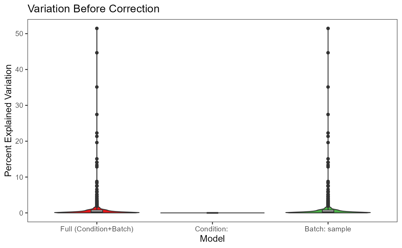

plotBatchVariance(inSCE = sce.small, 
                  useAssay = 'LIMMA', 
                  batch = 'sample',
                  title = 'Variation After Correction')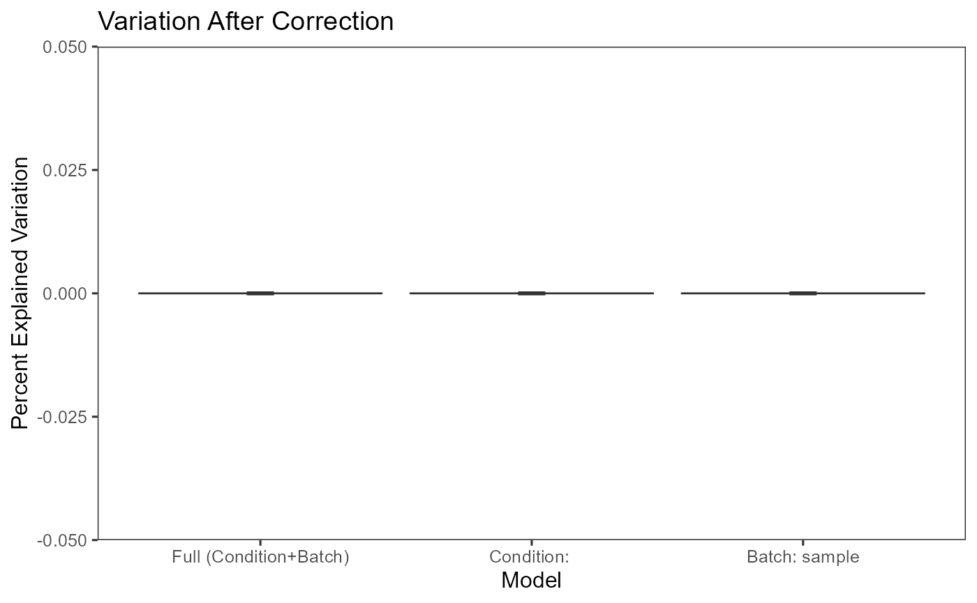

Plot the mean expression level of each gene separately for each batch.

This functionality is implemented in plotSCEBatchFeatureMean(). The methodology is straight forward, which plots violin plots for all the batches, and within each batch, the plot illustrates the distribution of the mean expression level of each gene. Thus the batch effect can be observed from the mean and standard deviation of each batch.

Plot a dimension reduced components to see the grouping of cells

There is no function special for batch correction, but this can be achieved simply by using the dimension reduction calculation functions (e.g. scaterPCA(), getUMAP() and getTSNE()) and plotSCEDimReduceColData().

sce.small <- scaterPCA(inSCE = sce.small,
                    useAssay = 'logcounts', 
                    reducedDimName = 'PCA')
plotSCEDimReduceColData(inSCE = sce.small,
                        colorBy = 'sample',
                        reducedDimName = 'PCA', 
                        title = 'PCA Before Correction')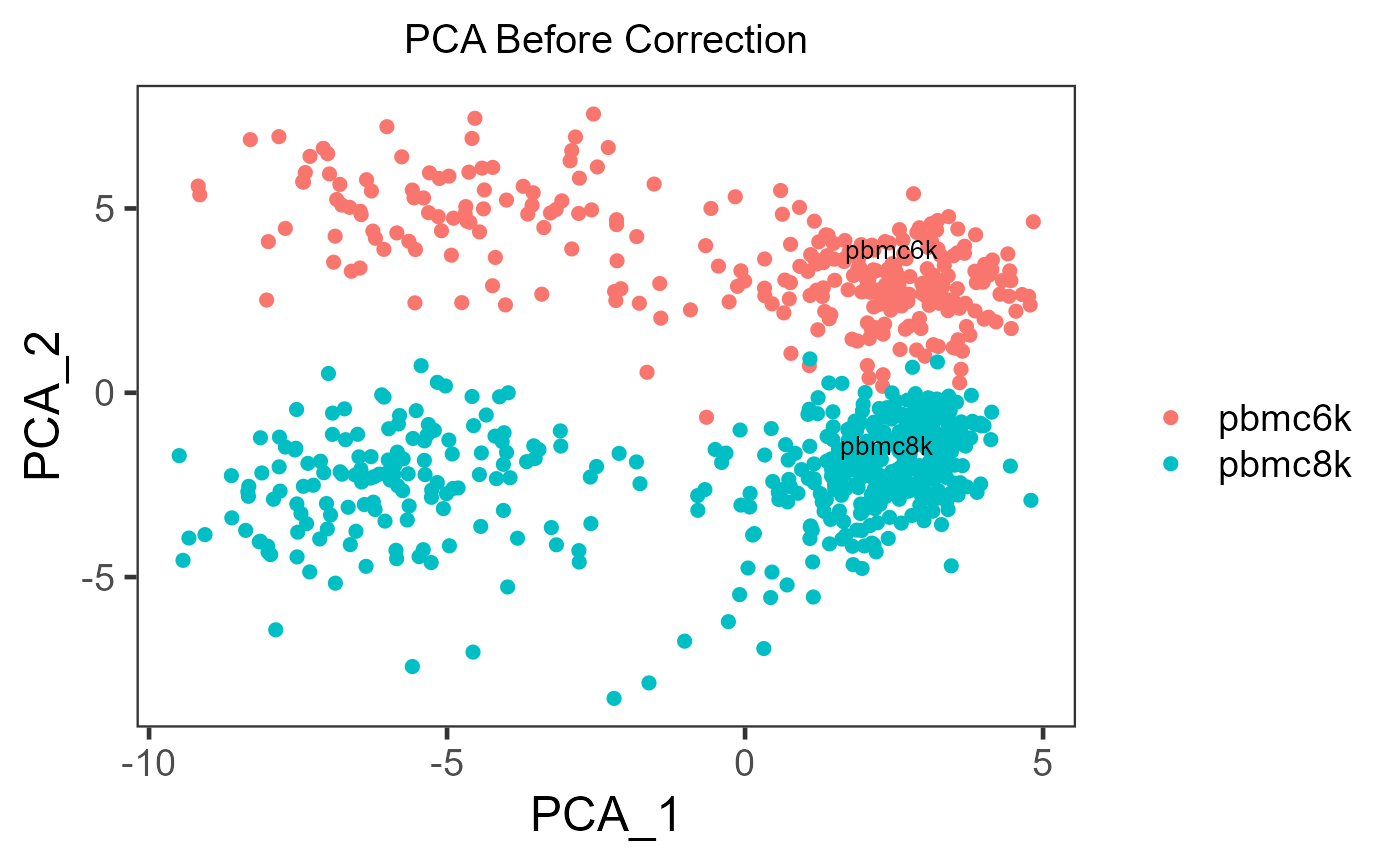

sce.small <- scaterPCA(inSCE = sce.small,
                     useAssay = 'LIMMA', 
                     reducedDimName = 'PCA_LIMMA')
plotSCEDimReduceColData(inSCE = sce.small,
                        colorBy = 'sample',
                        reducedDimName = 'PCA_LIMMA',
                        title = 'PCA After Correction')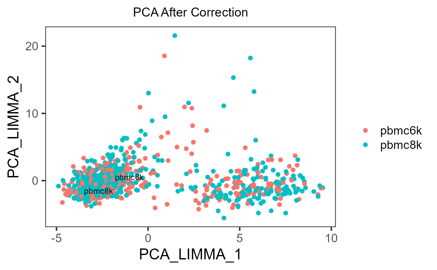

If the cell typing is already given, it is strongly recommended to specify shape = {colData colname for cell typing} in plotSCEDimReduceColData() to visualize the grouping simultaneously.