Dimensionality Reduction
Irzam Sarfraz
Source:vignettes/articles/dimensionality_reduction.Rmd
dimensionality_reduction.RmdIntroduction
Dimensionality reduction algorithms (PCA/ICA) can be run through the singleCellTK toolkit using both interactive shiny application and R console. For the interactive analysis, the toolkit offers a streamlined workflow to both compute metrics for dimensionality reduction and then visualize the results using any of the available interactive plots. For the console analysis, the toolkit offers a single wrapper function runDimReduce() to compute metrics for any of the integrated algorithms and multiple methods to visualize the computed results.
Methods available with the toolkit include PCA from scater [1] package and PCA & ICA from Seurat [2][3][4][5] package. Visualization options available for users include 2D Component Plot, Elbow Plot, JackStraw Plot and Heatmap. A complete list of supported visualization options against each method are specified at the bottom of the tabs below.
To view detailed instructions on how to use these methods, please select ‘Interactive Analysis,’ from the tabs below, for performing dimension reduction in shiny application or ‘Console Analysis’ for using these methods in R console:
Workflow Guide
In general, the UI offers options for selection of data items and choice of parameters on the left side, and a visualization panel on the right side of the interface. A detailed workflow guide to run and visualize dimension reduction (DR) is described below:
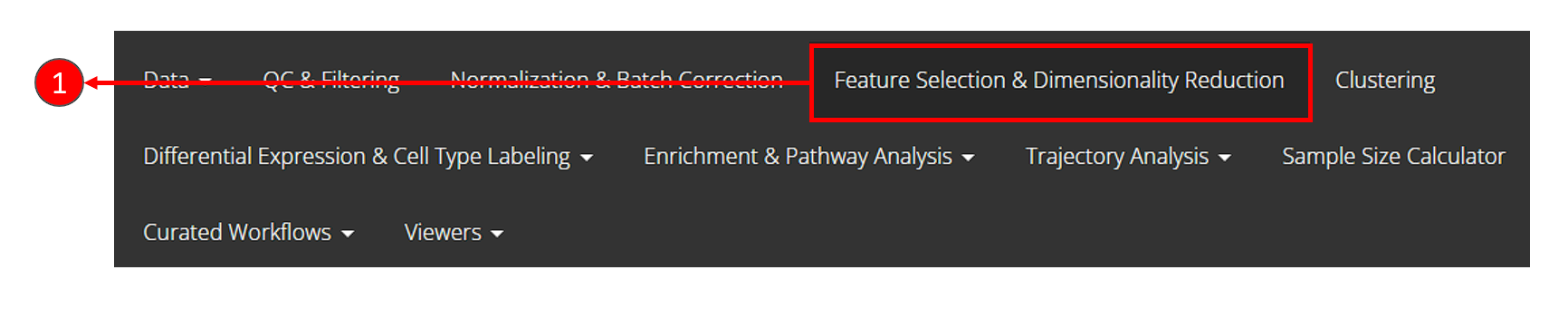
- To begin the DR workflow, click on the “Feature Selection & Dimensionality Reduction” tab from the top menu. This workflow assumes that before proceeding towards computation of DR, data has been uploaded, filtered and normalized (and optionally variable features have been identified) through the preceding tabs.
- Select “Dimensionality Reduction” tab:

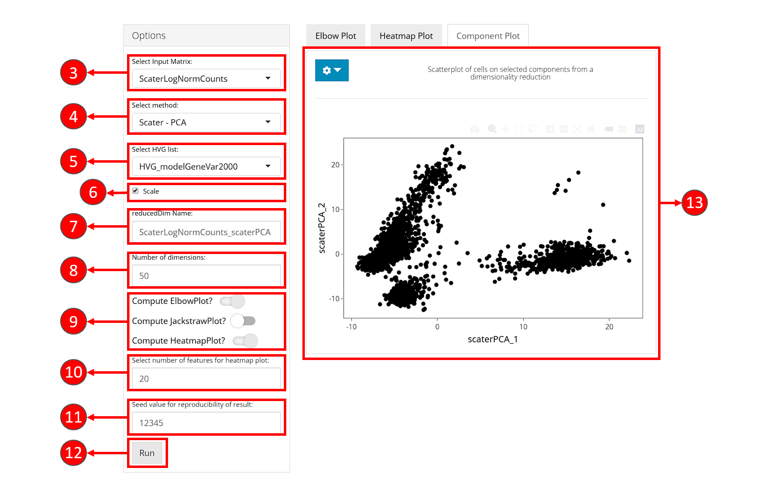
- Select an expression matrix which should be used for computation, usually log-normalized matrix is recommended.
- Select a method for dimensionality reduction. Available choices are “PCA” from scater package and “PCA” & “ICA” from Seurat package.
- (Optional) Choose a subset of features to use for dimension reduction. Subsets can be obtained from Feature Selection tab.
- (Optional) Check whether to scale the variance of features (subset of features if chosen in 5.) in the selected expression matrix before reducing dimensionality. Usually, scaling the subset of highly variable features is recommended.
- Specify a name for result low-dimensional data.
- Specify the number of dimensions to generate with the selected algorithm. Default value is
50. - (Optional) Check the boxes for optional visualization methods that should be applied after the computation of dimension reduction. Requested visualization will be shown in sub-tabs on the right side.
- If “Compute HeatmapPlot?” is selected in 9., you can specify how many features should be involved in the each heatmap. This setting can be changed later as well from the visualization panel on the right.
- Set the seed of randomized computation process. A fixed seed generates reproducible result each run.
- Press “Run” to start computation.
- Once processing is complete, selected visualization methods will be shown in the tabset on the right, together with the “Component Plot” (by default shown) which contains a scatter plot of cells on the top two components (dimensions).
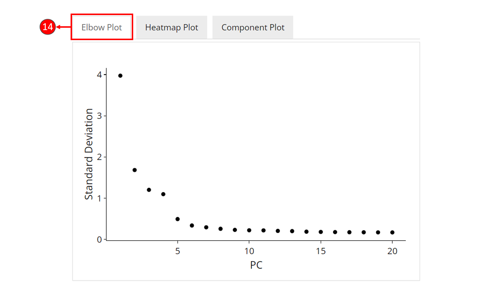
- An optional elbow plot can be computed for a PCA result, when chosen in step 9. It is a heuristic method which shows a relationship between the increasing number of components and the standard deviation. Components before an elbow break are empirically considered as containing most of the information of the data, and should be selected for downstream analysis.
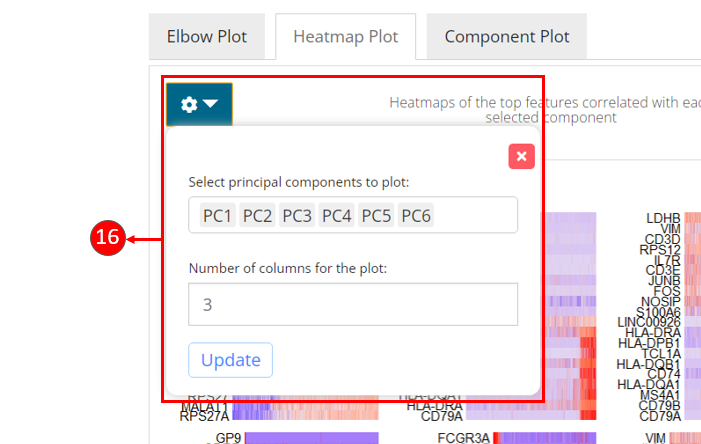
- Heatmaps can be computed optionally, when chosen in step 9. Each heatmap shows the expression of the features that are correlated to a component. This method allows for easy exploration of the primary sources of heterogeneity in a data set, and can be useful for determining number of components to include for downstream analysis.
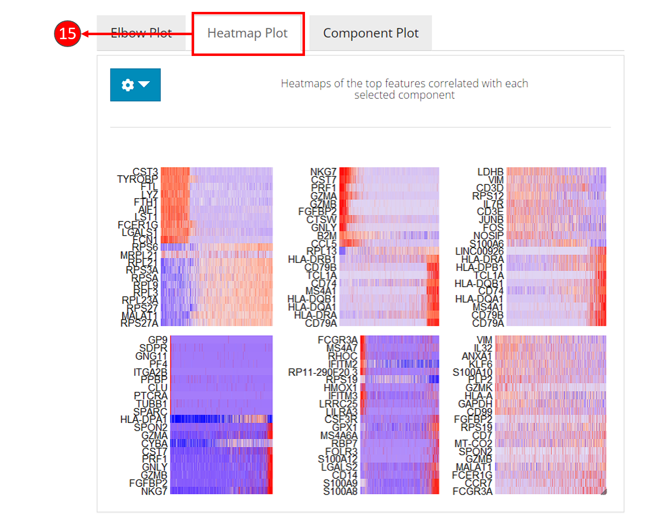
- Customization for the heatmaps can be made by selecting the components to display and entering the number of columns to organize the sub-plots.
Visualizations Supported
| Method | 2-Dimensional Component Plot | Elbow Plot | JackStraw Plot | Heatmap Plot |
|---|---|---|---|---|
| PCA | yes | yes | yes | yes |
| ICA | yes | no | no | yes |
Here we show how to perform dimension reduction with the generic function runDimReduce(), together with the method to visualize and explore the results.
1. Compute dimensionality reduction
sce <- runDimReduce(inSCE = sce, method = "scaterPCA", useAssay = "logcounts",
                    scale = TRUE, useFeatureSubset = "HVG_modelGeneVar2000",
                    nComponents = 50, reducedDimName = "PCA")
The generic function runDimReduce() allows "scaterPCA" from scater, "seuratPCA" and "seuratICA" from Seurat as options of dimension reduction for method argument. For detailed parameter description, please click on the function name to be redirected to its reference page.
2. Visualization
There are multiple functions that can create scatter plot using dimensions stored in reducedDims slot of the SCE object.
# Make scatter plot without annotation
plotDimRed(sce, useReduction = "PCA")
# Short-cut for reduced dims named as "PCA"
plotPCA(sce)
# Customizing scatter plot with more information from cell metadata (colData)
plotSCEDimReduceColData(sce, colorBy = "cluster", reducedDimName = "PCA")
# Color scatter plot with feature expression
plotSCEDimReduceFeatures(sce, feature = "CD8A", reducedDimName = "PCA")
Besides, SCTK also wraps elbow plot, Jackstraw plot and DimHeatmap methods from Seurat. For usage of these visualization methods, please refer to Seurat Curated Workflow
Example
library(singleCellTK)
sce <- importExampleData("pbmc3k")
sce <- runNormalization(sce, normalizationMethod = "LogNormalize", useAssay = "counts", outAssayName = "logcounts")
sce <- runFeatureSelection(sce, useAssay = "counts", method = "modelGeneVar")
sce <- setTopHVG(sce, method = "modelGeneVar", hvgNumber = 2000, featureSubsetName = "HVG")
# Run
sce <- runDimReduce(sce, method = "seuratPCA", useAssay = "logcounts",
                    scale = TRUE, useFeatureSubset = "HVG", reducedDimName = "PCA", nComponents = 50)
# Plot
plotDimRed(sce, "PCA")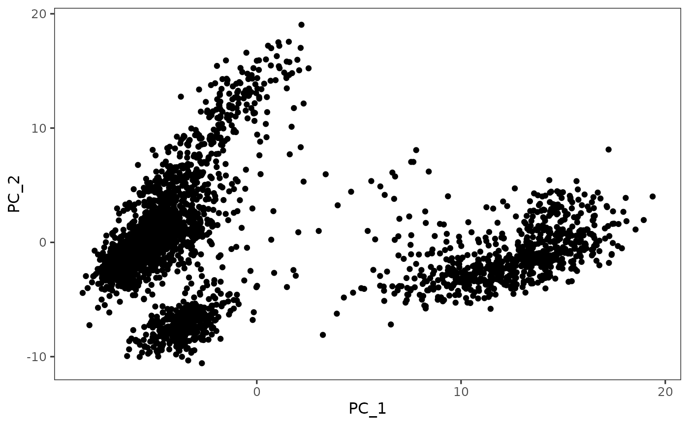
Individual Functions
While the runDimReduce() wrapper function can be used for all dimensionality reduction algorithms including PCA and ICA, and additionally for 2D embeddings like tSNE and UMAP, separate functions are also available for all of the included methods. The following functions can be used for specific methods:
Running PCA with Seurat method:
# Recommended to find variable features before running runSeuratPCA
# sce <- runSeuratFindHVG(inSCE = sce, useAssay = "seuratScaledData")
sce <- runSeuratPCA(inSCE = sce, useAssay = "seuratNormData", scale = TRUE, reducedDimName = "seuratPCA")
Running ICA with Seurat method:
# Recommended to find variable features before running runSeuratICA
# sce <- runSeuratFindHVG(inSCE = sce, useAssay = "seuratScaledData")
sce <- runSeuratICA(inSCE = sce, useAssay = "seuratNormData", scale = TRUE, reducedDimName = "seuratICA")
Running PCA with scater method:
# Recommended to find variable features before running scaterPCA
# sce <- runSeuratFindHVG(inSCE = sce, useAssay = "seuratScaledData")
# sce <- setTopHVG(inSCE = sce, hvgNumber = 2000)
sce <- scaterPCA(inSCE = sce, useAssay = "logcounts",
                 useFeatureSubset = "HVG_vst2000", scale = TRUE,
                 reducedDimName = "scaterPCA")
Visualizations Supported
| Method | 2-Dimensional Component Plot | Elbow Plot | JackStraw Plot | Heatmap Plot |
|---|---|---|---|---|
| PCA | yes | yes | yes | yes |
| ICA | yes | no | no | yes |