Dimensionality Reduction
Irzam Sarfraz
Source:vignettes/articles/cnsl_dimensionality_reduction.Rmd
cnsl_dimensionality_reduction.RmdIntroduction
Dimensionality reduction algorithms (PCA/ICA) can be run through the singleCellTK toolkit using both interactive shiny application and R console. For the interactive analysis, the toolkit offers a streamlined workflow to both compute metrics for dimensionality reduction and then visualize the results using any of the available interactive plots. For the console analysis, the toolkit offers a single wrapper function runDimReduce to compute metrics for any of the integrated algorithms and multiple methods to visualize the computed results.
Methods available with the toolkit include PCA from scater [1] package and PCA & ICA from Seurat [2][3][4][5] package. Visualization options available for users include 2D Component Plot, Elbow Plot, JackStraw Plot and Heatmap Plot. A complete list of supported visualization options against each method are specified at the bottom of the tabs below.
To view detailed instructions on how to use these methods, please select ‘Interactive Analysis’ for using normalization in shiny application or ‘Console Analysis’ for using these methods on R console from the tabs below:
Workflow Guide
In general, both sub-tabs offer options for selection of data items and choice of parameters on the left side, and a visualization panel on the right side of the interface. A detailed workflow guide to run and visualize dimensionality reduction (DR) algorithms is described below:
- To begin the DR workflow, click on the “Feature Selection & Dimensionality Reduction” tab from the top menu. This workflow assumes that before proceeding towards computation of DR, data has been uploaded, filtered and normalized (and optionally variable features have been identified) through the preceding tabs.

- Select “Dimensionality Reduction” tab:

- Select a data item (assay or a feature subset) which should be used for computation.
- Select an appropriate method for dimensionality reduction. Available choices are “PCA” from
scranpackage and “PCA” & “ICA” fromseuratpackage.
- Specify a name for the new data (reducedDim).
- Specify the number of dimensions to compute against the selected algorithm. Default value is
10.
- Check the boxes against the visualizations that should be plotted after computation of reducedDims. This visualizations become available after computation on the right panel.
- If “Compute HeatmapPlot?” is selected in step 8, you can specify how many features should be plotted in the heatmap by default. These setting can be changed later as well from the visualization panel on the right.
- Press “Run” to start computation.
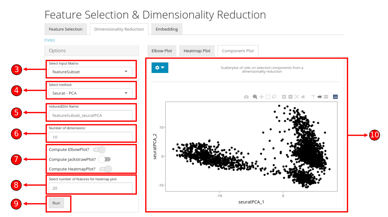
- Once processing is complete, selected visualizations appear in this panel. A 2D plot between the top two components is computed for all methods
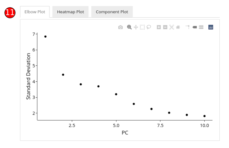
- Elbow plot (optional) can be computed against PCA methods. It shows a relationship between the increasing number of components and the standard deviation, where components before an elbow break should be selected for downstream analysis.
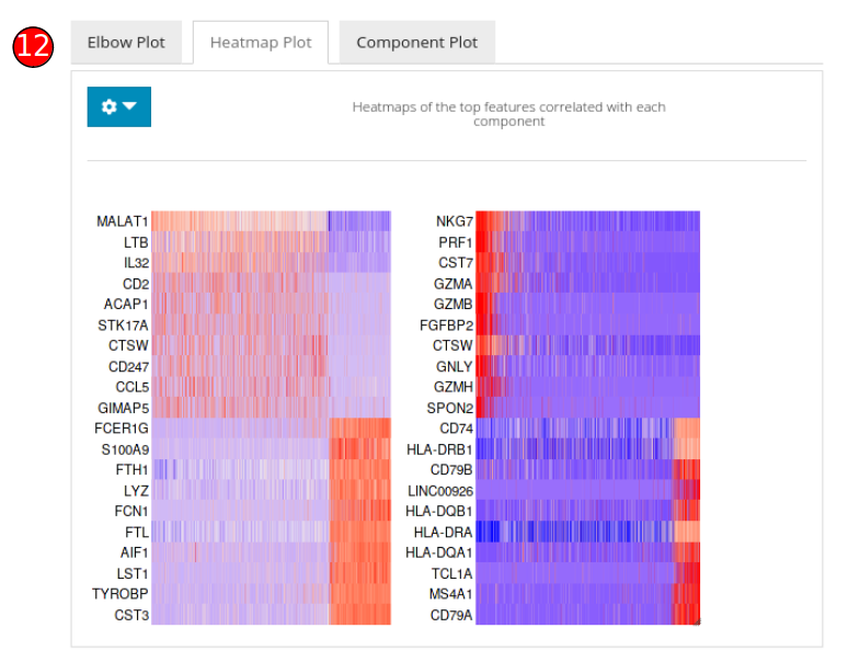
- Heatmap plot panel can be used to visualize the features against each of the computed component.
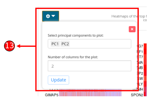
- Customizations for the heatmap plot can be made by selecting the components that should be selected. Number of columns for visualization can be specified as well for better viewing experience.
Note: Some parameters may differ between different methods and may not have been shown here.
Visualizations Supported
| Method | 2-Dimensional Component Plot | Elbow Plot | JackStraw Plot | Heatmap Plot |
|---|---|---|---|---|
| PCA | yes | yes | yes | yes |
| ICA | yes | no | no | yes |
In general, the first step is to compute a dimensionality reduction (e.g. PCA) and then the second step is to visualize the computed results. The usage of functions to compute and visualize results is described below.
1. Compute dimensionality reduction statistics using runDimReduce wrapper function:
sce <- runDimReduce(inSCE = sce, useAssay = "normalizedCounts", reducedDimName = "redDimPCA", method = "seuratPCA", nComponents = 20)To use the function, input a SingleCellExperiment object that contains the data assay and specify the required parameters (to see a complete list of supported parameters and to copy the function call against each method with the supported parameters, please view the ‘Parameters’ heading at the end of this page).
Function Call for Each Method:
scaterPCA:
sce <- runDimReduce(inSCE = sce, useAssay = "normalizedCounts", reducedDimName = "redDimPCA", method = "scaterPCA", nComponents = 10)seuratPCA:
sce <- runDimReduce(inSCE = sce, useAssay = "normalizedCounts", reducedDimName = "redDimPCA", method = "seuratPCA", nComponents = 10)seuratICA:
sce <- runDimReduce(inSCE = sce, useAssay = "normalizedCounts", reducedDimName = "redDimICA", `method` = "seuratICA", nComponents = 10)2. Visualize the dimensionality reduction results through a scatterplot:
#To plot a simple 2D component plot for any of the 4 methods i.e. PCA, ICA, tSNE and UMAP
plotDimRed(inSCE = sce, useReduction = "redDimPCA", xAxisLabel = "PC_1", yAxisLabel = "PC_2")
Example
  # Load singleCellTK & pbmc3k example data
  library(singleCellTK)
  sce <- importExampleData(dataset = "pbmc3k")
  # Perform Normalization
  sce <- runNormalization(inSCE = sce, normalizationMethod = "LogNormalize", useAssay = "counts", outAssayName = "LogNormalizedScaledCounts", scale = TRUE, trim = c(10, -10))
  # Find Variable Features
  sce <- runFeatureSelection(inSCE = sce, useAssay = "counts", hvgMethod = "vst")
  sce <- getTopHVG(inSCE = sce, method = "vst", n = 2000, altExp = "hvg2000")
  # Run PCA
  sce <- runDimReduce(inSCE = sce, useAssay = "LogNormalizedScaledCounts", useAltExp = "hvg2000", reducedDimName = "redDimPCA", method = "seuratPCA", nComponents = 10)
  # Plot PCA
  plotDimRed(inSCE = sce, useReduction = "redDimPCA", xAxisLabel = "PC_3", yAxisLabel = "PC_2")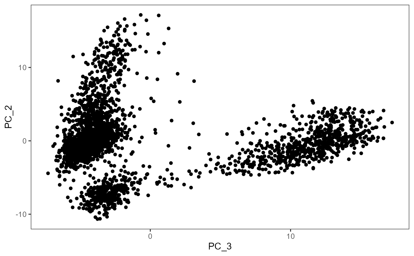
Parameters
The runDimReduce function takes in different parameters based on the specific method used for dimensionality reduction. See below for a complete description of parameters for each individual method in the runDimReduce function:
| Method | Parameters |
|---|---|
| scaterPCA |
inSCE (input SingleCellExperiment object), useAssay (name of the assay to use), useAltExp (name of the altExp slot if you want to compute on an altExp/subset/variable features instead of the main assay), reducedDimName (name of the computed reducedDim), method = “scaterPCA,” nComponents (number of components to compute, default is 10) |
| seuratPCA |
inSCE (input SingleCellExperiment object), useAssay (name of the assay to use), useAltExp (name of the altExp slot if you want to compute on an altExp/subset/variable features instead of the main assay), reducedDimName (name of the computed reducedDim), method = “seuratPCA,” nComponents (number of components to compute, default is 10) |
| seuratICA |
inSCE (input SingleCellExperiment object), useAssay (name of the assay to use), useAltExp (name of the altExp slot if you want to compute on an altExp/subset/variable features instead of the main assay), reducedDimName (name of the computed reducedDim), method = “seuratICA,” nComponents (number of components to compute, default is 10) |
Individual Functions
While the runDimReduce wrapper function can be used for all dimensionality reduction algorithms including PCA/ICA & additionally for tSNE/UMAP, separate functions are also available for all of the included methods. The following functions can be used for specific methods:
PCA from Seurat package:
  # Recommended to find variable features before running runSeuratPCA
  # sce <- runSeuratFindHVG(inSCE = sce, useAssay = "seuratScaledData")
  sce <- runSeuratPCA(inSCE = sce, useAssay = "seuratScaledData", reducedDimName = "seuratPCA", nPCs = 20, verbose = TRUE)
The parameters to the above function include: inSCE: an input SingleCellExperiment object useAssay: name of the assay to use for PCA computation reducedDimName: name of the computed PCA reducedDim nPCs: a numeric value indicating the number of components to compute verbose: a logical value indicating if progress should be printed
ICA from Seurat package:
  # Recommended to find variable features before running runSeuratICA
  # sce <- runSeuratFindHVG(inSCE = sce, useAssay = "seuratScaledData")
  sce <- runSeuratICA(inSCE = sce, useAssay = "seuratScaledData", reducedDimName = "seuratICA", nics = 20)
The parameters to the above function include: inSCE: an input SingleCellExperiment object useAssay: name of the assay to use for ICA computation reducedDimName: name of the computed ICA reducedDim nics: a numeric value indicating the number of components to compute
PCA from Scater package:
sce <- scaterPCA(inSCE = sce, useAssay = "logcounts", reducedDimName = "PCA", ndim = 50, scale = TRUE, ntop = NULL)The parameters to the above function include: inSCE: an input SingleCellExperiment object useAssay: name of the assay to use for PCA computation reducedDimName: name of the computed PCA reducedDim ndim: number of principal components to obtain from the PCA computation scale: logical value indicating whether to standardize the expression values ntop: number of top features to use as a further variable feature selection
Visualizations Supported
| Method | 2-Dimensional Component Plot | Elbow Plot | JackStraw Plot | Heatmap Plot |
|---|---|---|---|---|
| PCA | yes | yes | yes | yes |
| ICA | yes | no | no | yes |